Assimilation of meteorological data

Meteorological observation tools (satellites and ground stations) provide a very large amount of meteorological data, which must be processed to establish the state of the atmosphere from the forecast model. It is this processing that is called data assimilation. It must result in a value of each of the atmosphere parameters in each grid cell of the model. This initial step in weather forecasting is crucial because any initial error has the property of spreading and gradually contaminating the entire atmosphere.

1. The challenge of the starting point for a weather forecast

To predict the weather, major weather centres use a prediction model that simulates the evolution of the atmosphere for the coming hours or days. This model uses fluid mechanics equations (see Weather forecasting models), which are evolutionary equations in time: knowing the solution at a given moment, we can obtain their solution at any future moment. These equations are combined with others such as those that characterize changes in the state of water in the atmosphere or interactions with the Earth’s surface.

Weather forecasts are therefore obtained by running these forecast models over a given time period, but it is still necessary to know the starting point. To do this, we rely on data assimilation, which makes it possible to pass from meteorological data, collected at the moment of the starting point, to the values of the model parameters at the same moment but for each of its elementary meshes.

2. Meteorological data

The atmospheric observing system we know today has been developed over the last few centuries, but the invention of radiosondes in 1928 provided a first decisive dataset, providing a way to probe the three-dimensional structure of the atmosphere. The Second World War accelerated the deployment of a global network of radiosonde measurements in addition to ground-based measurements. The establishment of the World Meteorological Watch in 1963 also made it possible to establish a remarkable structure, aimed at maintaining a network of meteorological measurements on a global scale and ensuring the availability of these data in real time for all members of the World Meteorological Organization (WMO).

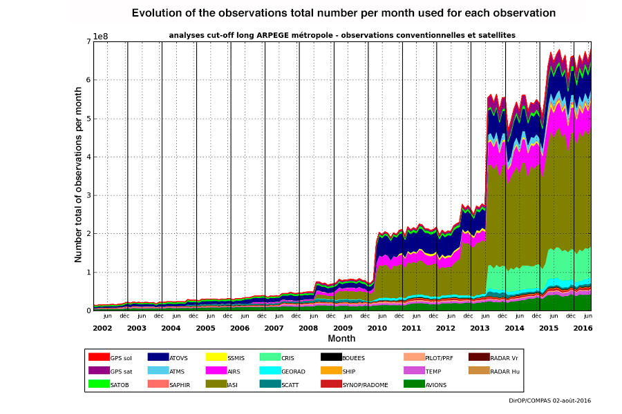
The so-called conventional data nowadays include observations provided by ground stations, radiosondes, sensors on airliners and commercial vessels or installed on anchored or drifting buoys. But these data now represent only about 10% of the total volume because 90% of the data is now provided by satellites (Figure 1). The growth in the number of data collected is very rapid (Figure 2) due to the permanent increase in the data provided by satellites. The number of data used by Météo-France to make forecasts for the entire globe is now around 20 million per day.

3. A brief history of data assimilation

In the first attempts at numerical weather prediction, Richardson in 1922 [1] and Charney in 1950 [2] plotted the meteorological data collected for a given parameter (e. g. temperature near the ground) and then manually plotted isolines of that parameter (e.g. contour lines on a geographical map) and finally transformed these isolines into numerical values for each mesh of the forecast model. This time-consuming process is not possible today.

Subsequently, different techniques were proposed to automate this manual process. One of these techniques was based on the idea that the value of a model parameter for a given point can be evaluated by averaging the measurements of the same parameter available around that point and giving less weight to the most distant measurements. Although providing a draft of the value of the model parameters for the starting point of the forecast, this type of method suffered from a number of limitations that were subsequently removed and are discussed in the following paragraphs.

4. How to find the most likely values of meteorological parameters?

In fact, the data on meteorological parameters collected around the globe are imperfect. Most often, they give an indication of the true value of a meteorological parameter at a given location and time, but with an error range that depends on the instrument that provided this data. For example, it is known that the measurements provided by the temperature sensors of the terrestrial network have a relatively small error range, but that on the contrary some observations provided by instruments on board satellites can provide measurements that deviate much more from the actual values. These errors are also random and therefore unknown at the time of measurement. This means that, even if data is available for a mesh of the model at the starting point of the forecast, this initial state will most often be wrong, which will limit the quality of the parameter forecast at subsequent times.

In order to overcome this uncertainty in meteorological measurements, one of the main ideas of data assimilation is to combine several measurements at a given point to obtain a better estimate of the true value of the desired parameter. On the other hand, we will try to make this combination the best possible. The chosen combination is a weighting of the different data available with weights directly related to what is called the accuracy of a measurement. This accuracy is simply defined as the inverse of the average amplitude of the squares of the deviations between the measurement provided by an instrument and a standard instrument without error. The variance of measurement errors associated with a given instrument is also referred to in statistical terms. An instrument with a high variance of measurement errors will therefore have low accuracy and, on the contrary, high accuracy if its variance of observation errors is low. It is therefore easy to see that the combination chosen will give more weight to precise observations than to imprecise ones.

5. A least squares problem

The best estimator is the solution of a weighted least squares problem. Such an approach was proposed almost simultaneously by Legendre [3] and Gauss [4] a little over two centuries ago. Applied to our estimation problem, this method is like searching for the values of a parameter for all the meshes of the model that are as close as possible to the available measurements. This can be achieved by minimizing the sum of the squares of the differences between these estimated values and the measurements, hence this least square expression. In order to take into account the expected amplitudes of the different measurements, each of these squared deviations is weighted by the variance of the errors of each of the measurements.

However, this approach only makes sense if the number and geographical distribution of available measurements coincide, at a minimum, with those of the values being sought (the value of one or more parameters for all the grid cells of the model). In practice this is not the case, even with the rapid increase in the number of measurements, because there is simultaneously another rapid evolution aimed at increasing the number of elementary meshes, in order to represent meteorological phenomena in an ever more precise way. It has already been indicated that today the number of measurements available over a 6-hour time range is in the order of a few million, while the number of variables for all the meshes of a forecast model is more in the order of a billion! Fortunately, this major indeterminacy can be overcome by implementing an appropriate algorithm that combines the available measurements with another source of information.

6. A continuous cycle of forecasts / corrections

The idea of combining the measurements with a draft solution provided by a recent forecast of the desired state is similar to the algorithm proposed by Kalman [5] and called the Kalman filter. A first major application of such an algorithm appeared in the 1960s for trajectory optimization problems in the context of the Apollo program.

This algorithm is based on a regular cycle of forecasts followed by corrections by the latest available measurements. For numerical weather prediction centres, this cycle is typically repeated every 6 hours for prediction models over the entire globe (such as the ARPEGE global model). It is generally shorter for finer scale models focused on a particular area of interest (1 hour for the AROME model focused on France). The correction or update phase consists of first calculating the differences between the forecast and all available observations. These gaps are called innovations, since they provide a source of innovation in relation to the forecast. The correction to the forecast is then obtained as a weighting of innovations using the same principles as the statistical linear estimate presented above. The weights given to each of the gaps between measurements and the forecast will thus depend on the relative accuracy of these measurements, but also, and this is the great novelty introduced by the Kalman filter, on the average amplitude and spatial structure of the forecast errors.

In the most complete form of the Kalman filter, as it can be used for small problems, the algorithm also provides a way to obtain an estimate anywhere of the accuracy of the resulting forecasts. However, this is unfortunately not possible for very large problems encountered in numerical weather forecasting because the number of calculations required becomes too high. We will see a little further on how we can get closer to this estimate of forecast accuracy at a lower cost.

From the moment a forecast and measurements are combined, it is easy to see that the question of the indeterminacy of the least squares problem raised in the previous paragraph disappears. Indeed, if the number of variables in the model to be estimated is about one billion, adding the values provided by a forecast to the ten million measurements is like adding all at once the same billion parameters of the model. Thus, the number of available information (measurements + expected parameters) becomes much higher than the number of values we are looking for (model parameters at a time). The values provided by the forecast can also be considered as specific additional measures.

7. The notion of observation operator

To solve the problem of data assimilation, difficulties remain when trying to apply them to a field such as meteorology. One of these difficulties is linked to the fact that today many of the measures taken into account are not of the same nature as the variables manipulated by the forecast model. This is the case for most of the data provided by measuring instruments on board satellites. Most often, a satellite instrument measures radiation emitted from the surface or an element of the atmospheric column that it overhangs. To be able to compare these measurements with the model variables, it is therefore necessary to transform the model variables into radiation beforehand, by applying a specific calculation, called an observation operator. We know how to move from the temperature and humidity column under a satellite to the radiation emitted by that column. The use of these observation operators thus makes it possible to use a very wide range of measurements such as satellite data but also data measured by terrestrial radars, which are so-called active instruments emitting radiation that is reflected on rain or hail. The development of these observation operators has been a significant step forward in data assimilation.

8. Practical determination of the solution

To solve the least squares problem introduced above, a way has yet to be found to obtain the set of atmospheric variables that is as close as possible to the collected measurements. To take into account a measurement that does not directly correspond to one of the variables of the model, we must therefore first apply to this set of variables of the model the observation operator corresponding to this measurement and it is the result of this operation that we will compare to the assimilated measurement. We are therefore able to write the sum of the squared deviations between the model variables and the measurements, supplemented by the sum of the deviations from the model variables provided by the forecast. We thus find ourselves with a sum of squares of deviations including about ten million deviations from observations (in the case of a global model) and depending on one billion variables (all possible values of the variables of the model for each of the elementary grid cells of the model).

The goal is to find the set of variables in the model that makes this sum of squares as small as possible. We are thus looking for the minimum of this distance between the variables of the model and the measures (implicitly including the forecast), which is also often called function-cost, a term that we find in optimization problems, to which this least squares problem is actually related. Although the problem then being addressed contains an enormous number of possibilities, it fortunately appears that the minimum sought can be obtained by an iterative process, with a number of iterations that does not exceed 100. The iterative process is based on the use of minimization algorithms well adapted to these least squares problems. Such an approach is now used by all major numerical prediction centres. This type of algorithm is also called 3D-Var, 3D because it is a three-dimensional problem (3 spatial dimensions, x, y, z) and Var because such a method falls into the class of variational algorithms (where we are interested in the variations of a cost function).

9. Consideration of the time dimension

We have seen above that the very diverse nature of the measures collected today requires transforming the model variables, by applying observation operators to them, in order to be able to compare them with observations. In fact, the diversity of observations is further complicated by the fact that many observations are now carried out almost continuously over time, making it difficult to compare a set of model variables at a particular time (from which to launch a forecast over a few days) with the data carried out around that time.

An elegant approach was proposed and developed in the 1980s and 1990s to solve this difficulty.

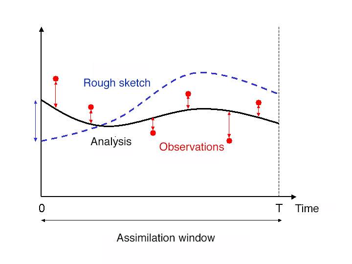
It consists in grouping observations over contiguous time intervals, called assimilation windows. For a global model, these assimilation windows usually last 6 hours and are centred on the so-called synoptic hours (0h, 6h, 12h, 12h, 18h), at which the radiosondes of the atmosphere are historically performed two or four times a day. Then, at the beginning of each assimilation window, we look for the set of variables in the model that gives the starting point of the forecast closest to the measurements throughout the assimilation window (this forecast is therefore made on the 6h of the assimilation window). This provides a state of the model variables that results from all the data collected during a given assimilation window and from which forecasts can then be made over several days.

This type of approach is always similar to a least squares minimization problem, which can still be solved by an iterative method. We speak of a 4D-Var, 4D approach because it is now a four-dimensional problem (3 spatial dimensions, x, y, z, and a temporal dimension t) (Figure 3). The implementation of 4D-Var algorithms has made it possible to take better account of observations, resulting in an improvement in the quality of forecasts.

10. Expected developments in data assimilation

The use of an increasing number of observations improves the quality of forecasts. This improvement is also largely due to the progress in data assimilation techniques. A particular effort is now being made to achieve a better representation of the uncertainty to be given to the forecast used in the forecast / correction cycle. To do this, the idea is to rely on the implementation of a set of such forecast / correction cycles, in which both sources of information (forecasting and measurements) are disrupted. The dispersion of the forecasts provided by such a set then makes it possible to quantify the uncertainty on the forecasts and is thus similar to the Kalman filter but at a reasonable cost. This is referred to as an ensemble Kalman filter (EnKF). Other important topics are also the subject of specific developments such as the best description of the uncertainties to be associated with the measurements. One of the focal points of the assimilation community is also the search for assimilation algorithms that will best lend themselves to an application on future generations of supercomputers that will include millions of processors!

 

---

References and notes

[1] L.F. Richardson, Weather prediction by numerical process, Cambridge University Press, Cambridge, Reprinted by Dover (1965, New York) with a new introduction by Sydney Chapman, 1922.

[2] Charney, J. G., R. Fjortoft, and J. von Neuman, Numerical integration of the barotropic vorticity equation, Tellus 2, 237-254, 1950.

[3] A.M. Legendre, Nouvelles méthodes pour la détermination des orbites des comètes, Paris, Firmin Didot, 1805.

[4] C.F. Gauss, Theoria Motus Corporum Coelestium, Ghent University, 1809.

[5] R.E. Kalman, A New Approach to Linear Filtering and Prediction Problems, Transaction of the ASME – Journal of Basic Engineering, Vol. 82, pp. 35-45, 1960.