On the contributions to statistical physics of Giorgio Parisi, Nobel Prize winner 2021

Three  Laureates  share  the 2021 Nobel  Prize  in  Physics  for  their  studies  of  complex  phenomena. Syukuro Manabe and Klaus Hasselmann laid the foundation of our knowledge of Earth’s climate and how humanity influences it. The third laureate, Giorgio Parisi is rewarded for his revolutionary contributions to the theory of disordered and random phenomena. In this article the authors Roberto Benzi and Uriel Frisch, close collaborators and friends of Giorgio Parisi, offer their vision of two of his major contributions, in which they have been respectively involved. Roberto Benzi explains the contribution of Parisi and collaborators to the conceptual understanding of the transitions from temperate to ice age climates. Uriel Frisch discuss one of the oldest unsolved problem in science, concerning the dynamics of turbulence and its proliferation of “fractals”.  The contributions of the two other laureates are presented in another article under the heading ‘climate’.

1.  A Nobel Prize for groundbreaking contributions to understanding of complex systems

While IPCC received the Nobel Prize of peace in 2007, climate science is honored by the Nobel price of physics for the first time in 2021. This science relies on classical fluid mechanics and thermodynamic processes, apparently far from the current frontier of physics. The difficulty however arises from the complex interaction of these various processes, occurring over a huge range of scales in space and time.

Among the three laureates, Syukoro Manabe and Klaus Hasselmann pioneered the modeling approach that led to the current climate models (read “On the contributions to climate sciences of Klaus Hasselmann et Syukuro Manabe, Nobel prize winner 2021”). This required a good physical insight to evaluate the dominant effects with very limited computer power. A more fundamental limitation is due to the unstable behaviour of the system, exemplified by the difficulty of weather forecast, even with the most powerful computers available nowadays. However such a chaotic behaviour leads to well defined statistics on long time scale, as requested for climate studies. This is the realm of statistical physics, the field of research to which Giorgio Parisi has provided several important contributions.

Statistical physics was initially developed to derive the properties of matter from first principles. After the pioneering contributions of Ludwig Boltzmann who clarified the concept of entropy, Albert Einstein and Paul Langevin quantified the Brownian motion of colloidal particles under the effect of random molecular collisions. Klaus Hasselmann has applied similar approaches to the climate systems, in which fast weather fluctuations replace molecular collisions. Giorgio Parisi and colleagues has analysed how such fluctuations trigger transitions between two stable states, as discussed in section 2.

Section 3 deals with a different topic, the old problem of turbulence, an intricate interaction of eddies at different scales which has defied physics and mathematics for more than a century. Giorgio Parisi introduced the concept of multifractals to account for experimental data.

Note that these two topics are not the only contributions for which Giorgio Parisi received the Nobel Prize. His most famous work is the theory of disordered magnetic systems, as explained by the official reports [1] of the Royal Swedish Academy. His various contributions provide insight in complex systems beyond physics. They also influence mathematics, biology, neuroscience and machine learning. This influence was favoured by his stimulating and friendly leadership among students and colleagues.

2. Stochastic resonance and interglacial periods (by R. Benzi)

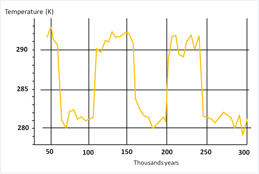
Scientists analysing the ice composition in Greenland and Antarctica provided good evidence that, during the last million years or so, Earth’s climate experienced glacial and interglacial periods with a periodicity of about 100,000 years and a temperature difference of about 10 degrees. It was a challenging question how to explain the observed quasi-periodic alternation of climate behavior (read “Astronomical theories of climate: a long history”).

To fix the question, let us consider the simplest possible climate model which deals with the global Earth energy budget (see figure 1). Sun provides incoming radiation (R_in) which is partly reflected (R_out) to the space by Earth’s surface (ice, clouds and other surface effects). The net incoming radiation R_in-R_out warms up Earth’s surface which emits infrared radiation. Knowing this net incoming radiation, one can estimate the ground temperature (on a global scale) using our knowledge on how radiative emission depends on temperature. In a stationary state, this infrared radiation just balances the net incoming radiation R_in-R_out. This provides a rather good estimate of the Earth mean global temperature corresponding to the present interglacial period around 15 degrees Celsius (read “The average temperature of the Earth”).

Although the emitted infrared flux is partly absorbed by green house gas in the atmosphere, the net emission is an increasing function of temperature, close to the black body expression in T⁴(read “The thermal radiation of the black body”). This is sketched as a linear function of T in figure 2. As for the reflected radiation, it strongly depends on the area covered by snow, which reflects light more efficiently than ground and free water. Therefore the incoming flux R_in-R_out also increases with temperature. As shown by Budyko [2] and Sellers, this increase is rather sharp with the melting of large ice cap over North America and Eurasia. This result in the black curve shown in figure 2.

Stationary states correspond to the three intersections of the two curves. The middle point represents however an unstable state: a small increase of temperature away from this stationary point indeed leads to an excess of incoming radiation R_in-R_out, resulting in a further increase of temperature, until the system reaches the warm stable point. Similarly a slight decrease of temperature is amplified and leads to the cold stable point representing a glacial climate. Therefore this model provides a simple conceptual explanation of two stable states.  In the original Budyko-Sellers model the glacial state referred to ice-covered Earth. It corresponds to extremely low temperature, never observed in paleoclimatic records of the last million years.

In the late 1920s the Serbian geophysicist Milutin Milanković performed an accurate and cumbersome computation of the Earth orbital variation around the Sun. He discovered that due to the eccentricity variation, the global incoming radiation was changing with approximately 100,000 years cycle. It was later discovered by John Imbrie and others that oscillation of the incoming sun radiation, as computed by Milanković, was almost in phase with the paleoclimatic Earth temperature during the glacial-interglacial oscillations.

At first sight, one may think that the Milanković cycle is able to explain the observed almost periodic behaviour in paleoclimatic records. However, there was a major problem puzzling scientists for decades: the point is that the Milanković fluctuations in the solar incoming radiation was extremely weak, of the order of 0.1 percent. This very small modulation of R_in-R_out would lead to a temperature modulation of about 0.2 degree, much smaller than the recorded temperature difference between glacial and interglacial states.

In the early eighties, Giorgio Parisi and his co-workers developed a new theoretical approach to solve the puzzle [3]. The starting point was again the surface energy budget previously considered. Next, looking at climate records and numerical circulation models, they understood that the Earth mean temperature is fluctuating from year to year due to internal and nonlinear dynamics of the climate. The crucial point was to consider these fluctuations as “noise” and in particular “internal noise” embedded in climate dynamics. Parisi and co-workers went on with this idea and observed that if there exist two climate states with a temperature difference of about 10 degrees, than Earth climate, due to internal climate fluctuations, can exhibit a random excursion from one state to another. This would randomly occur once every 50,000 years in average if the two states correspond to the observed glacial and interglacial states. This fits with the typical interval of 50 000 years between transitions, but without the true periodicity observed in paleoclimatic records.

The existence of two states can be understood, again, as the change of the out coming reflection of Earth surface as a function of temperature: upon decreasing temperature, it is no hard to imagine an increase of both ice and cloud cover in the climate and an equilibrium climate state can be reached.

The final step was to consider the effect of Milanković cycle on the system. At this point they discovered what is now called the mechanism of stochastic resonance: even if small, the Milanković cycle was able to change the probability of a transition from the present interglacial climate to the glacial state. These transitions were occurring almost in phase with the Milanković cycle. Indeed the probability of transition exponentially decreases with the distance to the intermediate unstable state, so a small reduction of this distance by the Milanković cycle is sufficient to strongly favour the transition. In figure 3 we show the temperature behaviour in the model used in the original publication [3] of Benzi, Parisi, Sutera and Vulpiani.

Beside the highly non trivial point concerning the existence of two climatic states (glacial and interglacial), the theory proposed by Parisi and coworkers is based on two fundamental concepts: noise effects on long time scales and noise-forcing cooperation.

For the first time in climate theories, noise was providing the driving mechanism for climate change on very long time scales. In climate, what we call noise is the effect of small scales nonlinear climate variables on the so called “coarse-grained” variables like the Earth global temperature. By now there are well defined and quantitative examples which allow us to speak of noise even if the word by itself can be misleading. The effect of the noise makes any system to perform fluctuations around some stable state (if it exists). However, if the system is non-linear and there exist more than one stable state, noise, with an exponential small probability, can drive the system from one state to another. Although small, on a very long time scale, as in the climate case, one should observed random (non-periodic) transition among the states.

The second point, namely cooperative effects of noise and external forcing, was entirely new in physics not only within climate theorists: nobody ever thought about this possibility. The paper[3] by Parisi and colleagues shows for the first time that this cooperation may occur in non-linear system like Earth’s climate. Later on, this cooperative effect was generalised for chaotic system [4] and, by now, there exist thousands of applications which exploit the mechanism of stochastic resonance in physics, biology and other scientific research.

3. Multifractal models for turbulence (by U. Frisch)

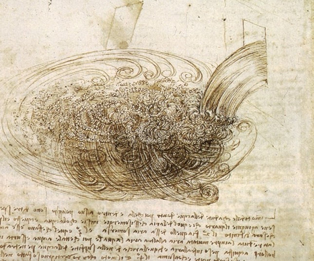
The very similar aspect of turbulent motion in air or water already interested Lucretius at the time of the Romans.  In the early 16^th century, Leonardo da Vinci studied the decay of eddies in rivers, see figure 4. All this makes turbulence one of the oldest unsolved problems in science.

Here, we begin with the oldest contribution, directly relevant to the work of Giorgio Parisi, namely that of A.N. Kolmogorov (1941) [5], abbreviated as K41. It deals with “fully developed turbulence”, which means that eddies can freely interact over a wide range of scales. These interactions transfer energy to very small eddies, which are damped by viscosity. This so-called energy cascade is at stake for instance in the process of turbulent drag (read “Drag suffered by moving bodies”). Specific flow features at the largest scales get scrambled by turbulent interactions through this cascade process. Kolmogorov then observed that, ignoring viscosity all the way together could lead to a dynamical equation in which the smaller and smaller eddies would just be similar – in a statistical sense – to those governing larger eddies. The correct level of similarity is determined by demanding a finite energy dissipation rate as the viscosity tends to zero. This self-similar picture (cf. figure 5, left) had an amazing success.

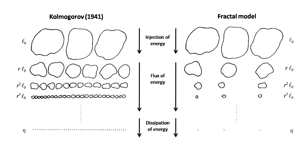
Although Kolmogorov was foremost a mathematician, one of the greatest in the 20^th century, he wanted to confirm his theory by experimental data collected in his Moscow laboratory and nearby. Such work provided strong evidence that turbulence is far from the above self-similar picture: the small eddies are much less space-filling than the larger ones and display intermittency (cf. figure 5, right). This led Kolmogorov and collaborators to propose a model for intermittency in 1961 [6]

An intermittency phenomenon had also been discovered by G.K. Batchelor and A.A. Townsend (1949) [7] and the question arose whether this phenomenon would be or not compatible with the self-similar picture of K41. For describing Kolmogorov’s intermittency, B. Mandelbrot (1974) [8] proposed using his “fractal” model. Fractals are geometrical objects obtained by iteratively inserting a similar pattern at smaller and smaller scales. Mathematicians had introduced this concept since the end of the 19^th century. In 1950, L.F. Richardson, another giant of turbulence and atmospheric dynamics, has used fractals in a completely different context, namely how to avoid conflicts between nations. It seems that a fractally convoluted border between countries will indeed be more prone to developing conflicts than a straighter one.

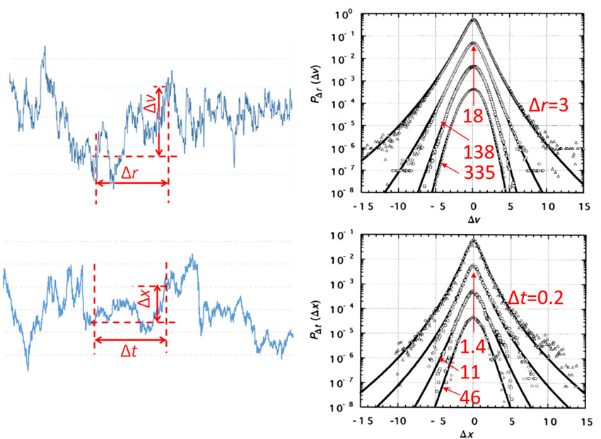
Returning to turbulence, a velocity probe crossing the turbulent field yields a typical “noisy” cut as shown in figure 6, top. Similar noisy signals are encountered in many complex systems, for instance financial markets (figure 6, bottom). They fascinate mathematicians as they are everywhere rough (the slope is not defined).

To grasp the multiscale structure of the signal, a natural approach is to study the velocity difference Δv between two points separated by a given distance Δr. The variance (the average of |Δv|²) indicates how the energy is distributed [9] among the different scales. However this is not the whole story: it does not distinguish rare and intense eddies from space-filling eddies with the same global energy. Such information is provided by the probability distributions (histograms) shown in the right hand side of figure 6. Long “tails” of these histograms represent rare and intense events. Those become stronger for small separation Δr, revealing the small eddies are rather sparse. This is the essence of intermittency. Similar analysis can be done for any time series by considering a time interval Δt instead of a distance, as shown in figure 6 for a financial market. Then the tails represent the probability of large drop or rise in a given time interval, which is of direct relevance for risk management.

Coming back to turbulence, these tails can be evaluated by considering the average of |Δv|^p (the moment of order p). Those are indeed more and more sensitive to large fluctuations as their order p is higher. Their dependency on the separation Δr, called the structure functions, therefore characterises intermittency. In the truly self-similar cascade described by K41, the structure function of order p behaves as the power law Δr^p/3 (figure 7). Experiments indicate a power law |Δr|^ζ(p) with exponents ζ_(p) smaller than p/3 :  high moments are relatively stronger in the limit of small separation Δr, which quantifies intermittency.

The model proposed by Kolmogorov in 1961 is closer to the experimental results, but it leads to a decrease of ζ_(p) for large index p which turns out to be mathematically inconsistent. As an alternative, fractal models making some contact with the dynamical equations for turbulence were introduced, particularly by Frisch, Sulem and Nelkin (1978) [10]. This yields a linear increase of ζ_(p) with p, with slope smaller than 1/3. The slope depends on a single parameter, such as the fractal dimension, quantifying how the active eddies get more and more sparse at smaller and smaller scales. Experiments however reveal a convex curve, as shown in figure 7.

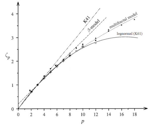
In the summer 1983, G. Parisi and U. Frisch attended a Varenna (Italy) summer school on “Turbulence and predictability in geophysical fluid dynamics and climate dynamics.” Experimental data by F. Anselmet, Y. Gagne, E.J. Hopfinger, R.A. Antonia [11] were hardly compatible with a single fractal, as shown in figure 7. With a remarkable physical intuition, G. Parisi suggested a multifractal model to account for these results. This agreement relies on fitting parameters but the underlying analysis revealed deep mathematical properties.

This idea of having more than one fractal dimension – even infinitely many fractal dimensions – has its origin in a very difficult subject: the evaluation of large risk or of financial ruin. The pioneering work had been done by a Swedish mathematician, H. Cramér (1938) [12] with strong background in finance. The standard vision before Cramér was that, by adding n independent and equally distributed random variables, one would get (with suitable conditions) two major properties : the mean would tend to the average (law of large numbers), and deviations from the mean, divided by n^1/2, would tend to a Gaussian law (the Central Limit Theorem).

But what happens when we multiply the variables instead of adding them (or equivalently when we add variables and take an exponential of the result)? This is precisely what happens in the pulverization of rocks, a problem studied by Kolmogorov [13] before the results of Cramér were well known. The probability of a given grain size indeed results from a product of probabilities of successive independent breaking events. It is then exceptional to obtain Gaussian limits. All these problems involve a strange function called the large deviation function, which characterises the deviation from the law of large numbers. The name changes depending on the field: “the rate function”, the “Cramér function” or the “entropy”. Yes, Boltzmann entropy is just a particular case; understanding entropy, without any advanced probability theory is remarkable, unless one is Boltzmann.

Here are some key references on multifractals. The initial reference is actually a 2.5 page Appendix by Parisi and Frisch to a paper by Frisch [14] published in the proceedings of the 1983 Varenna meeting.  Immediately following, a more detailed paper was written by Benzi, Paladin, Parisi and Vulpiani [15]. It included a crucial extension from fully developed turbulence to strange attractor in chaotic dynamical system. The key argument of these papers of the eighties make use of the Legendre transformation, the same transformation that appears in statistical thermodynamics when defining the entropy, but Cramér’s large deviations are not mentioned. A much more detailed presentation, centered on an elementary presentation of large deviations is in the book of Frisch (1995) [16]. Finally, there is an excellent online text by Y. Meyer (2021) [17], which is in principle intended for mathematician, but can be read also by persons without advanced mathematical knowledge.

We wish now to return to L.F. Richardson who was certainly aware of fractals already in the 1920s, when he introduced cascades in turbulence. Richardson borrowed a poem from Jonathan Swift, which is reproduced in figure 8 together with an illustration by Jérémie Bec. Unless the head-to-head distance between the left and the right fleas is made much smaller, the flea model is clearly fractal (and easily multifractal). As pointed out by Benoit Mandelbrot, fractals are quite common in natural phenomena and that is what we normally crave for. Mandelbrot objected against those making everything straight and rigid.

Finally, we want to stress a paradox. It is clear that increasingly accurate measurements of turbulent flow have been a driving force in the development of multifractal analysis. There are some solid theorems [18] concerning multifractal singularities arising in model equations. Nevertheless we do not have a single proven theorem applicable to Navier-Stokes equations, which describes three-dimensional (3D) strong turbulence. In spite of this precarious mathematical basis, multifractal analysis is now routinely used to quantitatively analyse a wide variety of complex chaotic or turbulent phenomena observed in the environment, like climatic time records, wind gusts, cloud shapes, solar wind.

4. Messages to remember

• Giorgio Parisi has been awarded the Nobel price of physics in 2021 for his leading contributions to major advances in statistical physics.
• Two of these contributions are relevant to climate and environmental flows. Those are the concepts of “stochastic resonance” and “multifractals”;
• Stochastic resonance is a cooperative effect of noise and external periodic forcing which can lead to nearly periodic switching between two stable states. It was initially proposed as a conceptual model for paleoclimatic records of the last million years but it turned out to have many applications in physics, biology and other scientific fields;
• Multifractals have been introduced to describe the multi-scale structure observed in turbulent flows. The concept turned out to have deep relevance for other chaotic systems and it triggered progress in the mathematical analysis of random processes.

 

---

Notes and references

Cover image. The three laureates of the Nobel Prize in physics, from left to right, Syukuro Manabe, Klauss Hasselmann, Giorgio Parisi [Source : © illustration Niklas Elmehed, Nobel Prize Outreach]

[1] Popular science background :  https://www.nobelprize.org/uploads/2021/10/popular-physicsprize2021.pdf , higher level version: https://www.nobelprize.org/uploads/2021/10/sciback_fy_en_21.pdf

[2] Budyko, M. I.  (1969) “The  effect of solar  radiation variations  on  the  climate  of  the  earth.”  Tellus 21, 611-619.

[3] Benzi R., Parisi G., Sutera A., Vulpiani A. (1982) “Stochastic resonance in climatic change”, Tellus 34, 10-16.

[4] Benzi R., Sutera A., Vulpiani A. (1981) “The mechanism of stochastic resonance”, J. Phys. A: Math. Gen. 14, L453-457.

[5] Kolmogorov, A.N. (1941a) “The local structure of turbulence in incompressible viscous fluid for very large Reynolds number”. Dokl. Akad. Nauk SSSR 30, 9-13 (translated in Proc. R. Soc. Lond. A 434, 9-13 (1991)).

[6] Kolmogorov, A.N.  (1961) “Précisions sur la structure locale de la turbulence dans une fluide visqueux aux nombres de Reynolds élevés”, in “La Turbulence en Mécanique  des Fluides”, 447-451, eds. A. Favre, L.S.G. Kovasznay, R. Dumas, J. Gaviglio & M. Coantic. Gauthiers-Villard, Paris. An English translation can be found in Kolmogorov, A.N.  (1962) J. Fluid Mech. 13, 82 – 85.

[7] Batchelor, G.K and Townsend, A.A. (1949) “The nature of turbulent motion at large wave-numbers”. Proc. R. Soc. Lond. A 199, 238-255.

[8] Mandelbrot, B. (1974) “Intermittent turbulence in self-similar cascades: divergence of high moments and dimension of the carrier”. J. Fluid Mech. 62, 331-358.

[9] This variance is related to the « energy spectrum » which can be obtained also from the Fourier transform of the signal.

[10] Frisch, U., Sulem, P.L. and Nelkin, M (1978) “A simple dynamical model of intermittent fully developed turbulence”. J. Fluid Mech. 736, 5-23.

[11] Anselmet, F., Gagne, Y., Hopfinger, E.J. and Antonia, R.A. (1984) “High-order velocity structure function in turbulent shear flow”. J. Fluid Mech. 140, 63-89.

[12] Cramér, H. (1938) “Sur un nouveau théorème-limite de la théorie des probabilités”, Actualités Scientifiques et Industrielle 736, 5-23.

[13] Kolmogorov, A.N. (1941) “On the logarithmic normal law of distribution of the size of particles under pulverization” Dokl. Akad Nauk SSSR 31, 99-101.

[14] Parisi, G. and Frisch, U. (1985) On the singularity structure of fully developed turbulence, in Turbulence and Predictability in Geophysical  Fluid Dynamics. Proceed Intern. School of Physics  ‘E. Fermi’. 1983. Varenna. Italy, 84-87.  This is an Appendix to the paper ‘Fully Developed Turbulence and Intermittency’ by Frisch, U. pp. 71-88.

[15] Benzi, Paladin, Parisi and Vulpiani (1984) “On the multifractal nature of fully developed turbulence and chaotic systems”, J. Phys. A: Math. Gen. 17, 3521.

[16] Frisch, U. (1995) “Turbulence, the Legacy of A.N. Kolmogorov”, Cambridge University Press.

[17] Meyer, Y. (2021) “Giorgio Parisi et la turbulence”,  Available in French on the site of the  “Institut national des sciences mathématiques et de leurs interactions” https://www.insmi.cnrs.fr/fr/cnrsinfo/giorgio-parisi-et-la-turbulence-par-yves-meyer .

[18] Jaffard, S. (2000) “On the Frisch-Parisi conjecture”, J. Math. Pures Appl. 69, 6, 525-552.