The average temperature of the earth

Global climate change is a major concern. It is based on the scientific community’s statement that human activities are the cause of a present and future global warming. But can we really define the average temperature of the planet and, if so, measure it? Can we really achieve an accuracy of a few tenths of a degree when we give the warming trends of the last century or when the international community set a target of limiting warming to only 2°C or even 1.5°C? Here we address the question of methodologies for determining the average temperature at the Earth’s surface, the accuracy of current reconstructions, and the questions of the observation and causes of its recent evolution.

1. Does the average global temperature make sense?

1.1. Link between energy balance and global temperature

The climate system (atmosphere, ocean, ice sheets, vegetation, etc.) receives most of its energy from the Sun (Figure 1) [1]. This energy received in the form of radiation corresponds roughly to the radiation of a black body with a temperature of about 5,800 K (Read Black Body Thermal Radiation), mainly in the visible range. As it passes through the atmosphere, some of this radiation is reflected or scattered by clouds, airborne particles (aerosols) and atmospheric gases. Another part of this radiation is absorbed by these gases and aerosols. Only part of the solar radiation reaches the surface, where it is also partly reflected. Therefore, only about half of the solar radiation incident at the top of the atmosphere (340W/m2) is absorbed at the Earth’s surface (160W/m2).

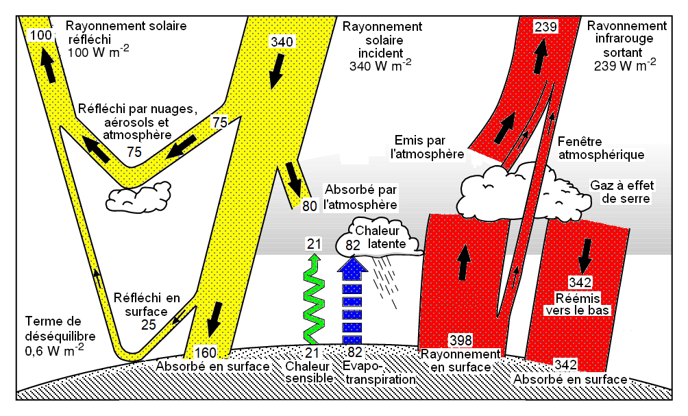
This energy input for the oceans and continents is, at equilibrium, compensated by an equivalent energy loss. This loss takes place either in the form of radiative energy, or in the form of heat transfers linked to conduction (known as sensible heat) or linked to phase changes in the water (known as latent heat). These energy losses are all a function of the Earth’s temperature, in particular the radiation emitted by the surface, which is close to that of a 288 K black body and is therefore in the infrared range.

It is to tend towards this energy balance at the surface, but also at the top of the atmosphere, that the Earth’s temperature is changing. But even if this physical mechanism is well known, the notion of a global average of the Earth’s temperature is not easy to grasp.

1.2. Average temperature? A statistical indicator!

The temperature of a solid, liquid or gaseous medium is a physical quantity that reflects the agitation of the particles that make it up in a given place. The sum of two temperatures therefore has no physical meaning. As a result, an average temperature over a wide range over which it varies from one place to another has no direct physical interpretation. This is therefore the case for the average temperature calculated over the entire surface of the Earth, covering both the warm tropical regions and the cold polar regions. However, this average is a statistical indicator that proves very useful for assessing climate change on a global scale, both in the past and in projection for the coming centuries. The global average temperature reflects changes in climate that can be explained by identifiable underlying physical mechanisms.

1.3. Example 1: Impact of greenhouse gases on the Earth’s average temperature

A first example is the average temperature difference that can be estimated by calculating the Earth’s energy balance due to the presence of naturally occurring greenhouse gases in the atmosphere. These gases have the property of absorbing the infrared radiation emitted at the Earth’s surface and then re-emitting some of it back to the surface, thereby further warming it (Figure 1). These include water vapour, carbon dioxide (_CO2) and methane (CH4) to name the main ones. Their contribution to the average global temperature is of the order of 33°C warming effect, bringing this temperature from about -18°C to +15°C.

It should be noted that this calculation only makes sense “all things being equal”, because if the Earth’s temperature were to cool by about 30 degrees, a change in the ice cover on its surface would result in additional cooling due to increased reflection of solar radiation (ice-albedo feedback effect).

1.4. Example 2: Effect of the Earth’s orbital parameters on its average temperature

Another example of a physical process resulting in a large deviation in the global mean temperature is primarily due to variations in the eccentricity of the Earth’s orbit. The Earth’s orbit around the sun is an ellipse whose eccentricity, measuring the deviation from its shape to that of a circle, varies between 0 (circular orbit) and 0.06 over the last million years with a main cycle of about 100,000 years. As eccentricity increases, the average distance from the Earth to the sun increases and thus the solar radiative energy received by our planet decreases. The result is a 100,000-year climate cycle of alternating cold (glacial) and warm (interglacial) periods over the last million years or so.

Understanding this 100,000-year cycle is still being researched because the direct effects of variations in the amount of energy received by the Earth are small. Some studies [2] show that it is also necessary to take into account the effects of variations in other astronomical parameters (obliquity, precession; see animation The drivers of natural climate evolution) and the physical effects amplifying temperature differences between cold and hot periods :

• The ice-albedo feedback effect already mentioned: the decrease in ice cover during warm periods reduces the reflectivity of solar radiation (the albedo) at the Earth’s surface, which contributes to increased warming by absorbing more radiative energy.
• The greenhouse effect because warm periods are also periods during which greenhouse gas concentrations increase as a result of physical processes and ecosystem changes.

The resulting global average temperature difference between the last cold period at its extreme (the last glacial maximum) about 21,000 years ago and the warm interglacial period we have known for about 10,000 years is thus likely between 3°C and 8°C [3].

Animation “The drivers of climate change” (Credit: Museum de Toulouse, Mercator Océan)

1.5. In summary

The global average temperature must therefore be seen as a statistical indicator of the evolution of the climate on the Earth’s surface. The two previous examples show to what extent this indicator can be sensitive to the physical and biological processes involved in the climatic balances of our planet, particularly those that have an effect on its energy balance.

Moreover, the second example, which corresponds to an observed change in the Earth’s climate, shows that a deviation of a few degrees in this indicator corresponds to very significant variations in climate. The few degrees less at the last glacial maximum correspond to much more extensive ice cover in the northern hemisphere (e.g. covering the northern part of the British Isles) and a sea level that is about 130 metres lower.

2. Reconstruction of global mean temperature from instrumental data

2.1. Observing the Earth’s surface

Assessing the average global temperature is a challenge. The accuracy of this estimate depends on the coverage of the Earth’s surface observation means, as temperature variations from one region to another can be significant. The study of the temporal evolution of the mean temperature also requires uninterrupted and homogeneous series of measurements, i.e. corrected for measurement disturbances linked in particular to changes in sensors or changes in the measurement environment.

If a few series of marine [4] and terrestrial [5] instrumental observations started in the 17th century, it was not until 1856 that the first meteorological observation network managed by Emmanuel Liais at Paris Observatory under the direction of the French astronomer Urbain Le Verrier [6] appeared. The reconstructions of the mean global temperature based on thermometric measurements thus date back to 1850 at the earliest.

Indirect reconstructions based on temperature estimates using natural archives (ice cores, sediment cores, tree rings, corals,…) and statistical models were also carried out by research teams. But, even if they cover much longer periods of time, they do not reach the accuracy or near-planetary coverage of the instrumental reconstructions to which we limit ourselves here.

2.2. The source data

Three main teams are behind the reconstruction of the global average temperature beginning in the second half of the 19th century. These are the American teams from the NASA Goddard Institute for Space Science [7], the National Oceanic and Atmospheric Administration (NOAA) [8] and the associated British teams from the Hadley Centre of the UK Met-Office and the Climate Research Unit of the University of East Anglia [9].

The source data are in part common to these three main reconstructions and are largely accessible:

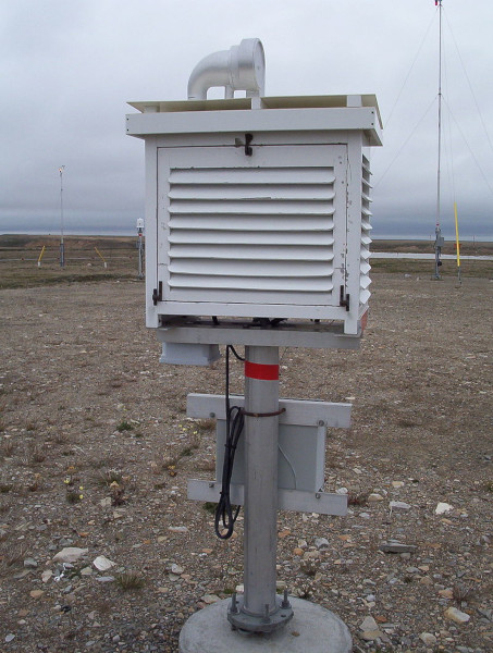
• For continental regions, these are the Global Historical Climatology Network [10] (GHCN) data from observations of sheltered air temperatures (Figure 2) from about 25,000 stations used in the NASA and NOAA reconstructions for the most recent version (GHCNv4).
• For marine regions, this is the International Comprehensive Ocean-Atmosphere Data Set [4] (ICOADS).

But while the American reconstructions use mainly GHCN data on the continent, the British reconstruction uses only part of it supplemented by data obtained directly from national meteorological services or other international climate databases [11]. On the other hand, the three reconstructions are essentially based on ICOADS marine data.

The continental temperature data used are measured in the air near the surface, now at a height of between 1.25m and 2m (1.5m in France) according to the recommendations of the World Meteorological Organization (See “Ground-based weather observations: what is measured and what is done with it?“). However, air temperature measurements measured on boats or buoys are less accurate than water temperature measurements due in particular to contamination of the sensors by salt and the difficulty of assessing the height of the measurement above the ocean surface in the case of boats. The authors of reconstructions have therefore chosen to evaluate the sea surface temperature not in the air but in the water (Figure 3). This choice has no impact on the study of the evolution of the global mean temperature as long as the calculation methods remain identical for the entire period of each reconstruction. However, it must of course be taken into account when estimating uncertainties (see 2.4).

Reconstructions of global mean temperatures depend on the collection and saving of data from old observations currently archived on documentary supports. The spatial and temporal coverage of the data can therefore be expected to improve in the future, especially for the most remote periods, as archived data such as those collected in the framework of the international I-DARE project are reprocessed [12].

2.3. Methods for calculating averages

Data are spatially dispersed and some regions remain poorly covered during the early stages of reconstruction. Conversely, some observations may be concentrated on certain regions, such as the European continent and the North Atlantic. It is therefore necessary to apply averaging procedures that take account of this spatial heterogeneity. The calculation procedures, which differ from one reconstruction to another, are precisely documented in scientific literature publications and we give only a very brief overview here.

For the British reconstruction, the available observations are averaged over a 5° latitude by 5° longitude grid, without any interpolation, before calculating a weighting average by the corresponding areas to obtain the global average [9]. For NASA, on the continent, the main intermediate step also consists of averaging on a terrestrial grid (of 8000 grids of equal areas), but weighted by the distance to the centre of each grid within a radius of 1200 km [7]. NOAA’s continental reconstruction is more sophisticated in that it involves interpolating (and extrapolating) the data using statistical functions that take into account the spatial correlations between observations (Empirical Orthogonal Teleconnection Functions or EOTs). The range of influence of these functions is limited to 2000 km in latitude and 4000 km in longitude around the centre of each grid [8]. It is also these statistical functions that are used in the American reconstructions to interpolate and extrapolate sea surface temperature data on a grid of 2° in latitude by 2° in longitude. In this case, the spatial domain of influence of the EOTs is limited to 3000 km and 5000 km respectively in latitude and longitude around the centre of each grid cell [13].

Finally, the data are calculated as deviations, or anomalies, from a climatic average (climatology) over a 30-year period, again a duration recommended by the World Meteorological Organization. The choice of reference periods is not the same for the three reconstructions (1961-1990 for the British and NOAA reconstructions; 1951-1980 for the NASA reconstruction), but this has no impact since we are only interested in the temporal evolution of temperature and not in its absolute value, which is difficult to interpret. One advantage of this is that it allows to overcome the differences in altitude of the stations taken into account for the calculation of the average in a given grid cell.

The reconstructions are available on grids covering the planet (5° by 5° for NOAA [14] and the British reconstruction [15], 2° by 2° for the NASA reconstruction [16]) and make it possible not only to calculate global averages but also to draw up maps of temperature trends over different regions. They are available in monthly and annual steps from 1850 for the British reconstruction and from 1880 for NASA and NOAA.

2.4. Estimation and error correction

Scientific articles and successive reports by the IPCC (Intergovernmental Panel on Climate Change) analyse the sources of error in reconstructions of global average temperature and, where possible, the methods used to correct them. Let us limit ourselves here to commenting on the main causes of errors, which are detailed in the focus “Error Calculation“. Some are related to sampling (number of observations per calculation grid cell) and incomplete coverage (absence of observations in some grid cells; Figure 4). The effects of urbanization around terrestrial observation stations result in an artificial warming trend that needs to be taken into account. Breaks in the homogeneity of the data series due to changes in the location of observation stations, instruments, weather shelters, or any other change that may affect the measurement, are also taken into account in the corrections of the reconstructions and in the associated error estimates. Marine data shall also be subject to corrections for bias due to changes in the means of observation used.

Globally, the uncertainty in the annual mean global temperature is calculated by combining all the errors or uncertainties that can be estimated, whether over the ocean or over the continent. Various estimates of the mean temperature are finally obtained, from reconstructions proposed by NASA [8], NOAA [9] and the British teams [10]. The estimates are very close from one reconstruction to another despite the different methodologies used. The main difference between the NOAA reconstruction and the other two is due to sampling and spatial coverage errors, with a priori a better consideration of Arctic data from the middle of the 20th century, which results in a decrease in uncertainty.

3. How and why has the average global temperature changed over the last two centuries?

3.1. Detecting trends

Figure 5, taken from an annual report of the World Meteorological Organization [17], shows the evolution of global mean temperature between 1850 and 2019 according to the three reconstructions introduced in section 2. The temperature values are calculated by removing for each reconstruction its average over the period 1981-2010 and are then represented in relation to a so-called “pre-industrial” reference (the HadCRUT4 average over the period 1850-1900 [9]). Two other estimates of the global mean temperature from re-analyses of data (here from the Japan Meteorological Agency [18] for JRA-55 and the European Centre for Medium-Range Weather Forecasting [19] for ERA5) are also shown in the Figure following the same procedure (see focus on “Surface temperature estimation by re-analyses“)

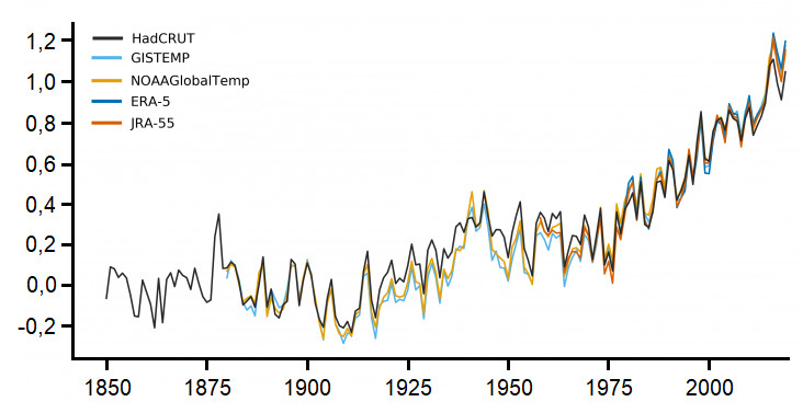
Figure 5 shows the very good agreement between the temperature changes resulting from the three reconstructions and the two re-analyses. The differences are perfectly compatible with the total uncertainties of each reconstruction. In particular, Huang et al [8] show that the British and NOAA reconstructions fall within the confidence interval of the NASA reconstruction each year (their Figure 13). The main differences arise firstly from the treatment of corrections for biases in ocean measurements during the period 1920-1960 [7], [9] (section 2.3). They also stem from the differences in spatial coverage of observed data and the way of treating poorly covered areas. In particular, the NASA and NOAA reconstructions take better account of Arctic data than the British reconstruction [7]. This has the effect of better reproducing the warming in these regions that has increased over the last few decades and which results in a slightly faster increase in global average temperature than is also observed in the re-analyses.

Figure 5 also highlights the superposition of different time scales of variability. The temperature trends calculated over the longest common period from the three reconstructions are very close to each other and clearly indicate a warming that is much greater than the uncertainties in each reconstruction. The latest IPCC Assessment Report [3] includes estimates of these trends and their calculated uncertainties up to the year 2012. According to this report, the global average surface temperature increased by nearly 0.9°C between 1880 and 2012 (with a 90% probability that the warming will be between 0.65 and 1.06°C). To get a good measure of this warming, it is sufficient to relate it to the 3-8°C warming between the last ice maximum (about 21,000 years ago) and the current period (see section 1). This warming trend has continued since this IPCC report, since between 1880 and 2018 the estimated trends are 0.96°C for NASA and NOAA (between 0.81°C and 1.11°C with a 95% probability according to [7]).

3.2. What is the observed warming due to?

The question of attributing all or part of this warming to greenhouse gas emissions emitted by human activities has been raised since the first IPCC report published in 1990. However, despite the observation of warming and the increase in atmospheric concentrations, particularly of carbon dioxide, already analysed at that time, no proof of a link had been provided and the report did not give any conclusion on attribution. Following the multiplication of studies providing evidence obtained by simulating the climate of the last century by varying the factors likely to influence temperature – natural with solar variability, volcanism and variability within the climate system or anthropogenic with greenhouse gas emissions and the production of airborne particles (aerosols) – successive IPCC reports have been increasingly assertive in attributing warming. The latest report [3] now concludes that it is extremely likely that human influence has been the main cause of the warming observed since the mid-20th century.

Figure 6 reproduces estimates of the contributions of different factors to the temperature trend over the period 1951-2010 and compares them with the observed trend. It highlights the small contribution of natural factors to the observed warming while the anthropogenic contribution is close to the observed one. On the other hand, the respective contributions of greenhouse gases (“GHG”) and aerosol particles (“OA”) are difficult to estimate precisely, as illustrated by the error “bars” surrounding these estimates.

3.3. How can temperature variability up to the multi-decadal scale be explained?

The anthropogenic effect is thus clearly demonstrated on a time scale of about 60 years. However, warming is not regular over this period and it is much more difficult to assess the anthropogenic contribution over a much shorter period. This can be explained by the presence of variability on a multi-decadal scale (over several decades) as shown in Figure 5 but also in Figure 7 which zooms in on the period 1950-2017 by combining the three reconstructions and the two re-analyses (with versions dating from 2018).

A first singular period is the one that extends from the 50s to the 70s. It is characterized by a relative stability of the average temperature despite the increase in greenhouse gas concentrations in the atmosphere. Distinguishing this anthropogenic contribution from the effect of other factors remains a challenge for such a short period of time. It should be noted, however, that several studies have shown a potential role of another anthropogenic effect, namely the increase in the concentrations of aerosol particles in the atmosphere, which may induce an otherwise observed reduction in solar radiation measured at the planet’s surface (global dimming). The rapid increase in temperature from the late 1970s onwards would then be explained in part by the effects of measures taken to limit emissions of sulphates and carbonaceous particles in industrialized countries which are also concomitant with an increase in solar radiation at the surface (global brightening) [20] [3].

Another example of multi-decadal variability leading to an attenuation of the warming trend concerns the period 1998-2012. Over this period, the temperature increase was only 0.06°C according to the HadCRUT4 reconstruction [3]. This is a period in which the increase in sea level and the increase in ocean heat content did not show a weakening. The origin of this slowdown in surface warming has been the subject of numerous publications in recent years and its precise interpretation remains a subject of scientific debate (see focus on “A look back at the “slowdown” in warming between 1998 and 2013“).

Finally, Figure 7 also shows temperature variability on an interannual scale that is also superimposed on long-term trends [21]. Although it is also not possible to assess the relative effect of all factors on the temperature of a particular year, an important natural factor can be identified at this scale. This is the occurrence of warm (El Niño) or cold (La Niña) events in the tropical Pacific Ocean. These episodes, which result from interactions between the ocean and the atmosphere, modify ocean surface temperatures over a period of several months and have a visible and similarly marked effect on global mean temperature as shown in Figure 7.

4. Messages to remember

• The average temperature of the Earth’s surface is changing in order to achieve a balance between the energy it receives and the energy it loses.
• Global average temperature is a statistical indicator that is particularly useful for assessing global climate change.
• From 1850 onwards, it can be estimated from monthly and annual step reconstructions using instrumental data from observations of air temperature on the surface of continents and water temperature at the ocean surface.
• Increasingly complex uncertainty models make it possible to account for the various sources of error in its estimation.
• According to the IPCC, the global average temperature has warmed by 0.9°C over the period 1880-2012, a warming far greater than the uncertainties in the estimates.
• It is extremely likely that human influence has been the main cause of the warming observed since the mid-20th century.
• However, it is not yet possible to quantify precisely the relative weight of the different contributions of natural or anthropogenic factors to the evolution of mean temperature on shorter time scales.

---

Notes and References

Cover image. How can we attribute an average temperature to the Earth, given the well-known variations according to latitude and season? [Source: Pixabay, copyright free images]

[1] Wild, M., Folini, D., Hakuba, M.Z., Schär, C., Seneviratne, S., Kato, S., Rutan, D., Ammann, C., Wood, E.F., König-Langlo, G. (2015) The energy balance overland and oceans: an assessment based on direct observations and CMIP5 climate models. Climate Dynamics, 44:3393-3429, DOI: 10.1007/s00382-014-2430-z.

[2] Abe-Ouchi, A., Saito, F., Kawamura, K., Raymo, M.E., Okuno, J., Takahashi, K., Blatter, H. (2013) Insolation-driven 100,000-year glacial cycles and hysteresis of ice-sheet volume. Nature, 500, 190-193, DOI :10.1038/nature12374.

[3] Climate Change (2013) The Physical Science Basis Contribution of Working Group I to the Fifth Assessment Report of the Intergovernmental Panel on Climate Change Stocker, T.F., D. Qin, G.-K. Plattner, M. Tignor, S.K. Allen, J. Boschung, A. Nauels, Y. Xia, V. Bex and P.M. Midgley (eds.)]. Cambridge, United Kingdom and New York, NY, USA: Cambridge University Press, 1535 pp. Available at: http://www.ipcc.ch/report/ar5/wg1/

[4] Woodruff, S. D., Worley, S. J., Lubker, S. J., Ji, Z., Freeman, J. E., Berry, D. I., Brohan, P., Kent, E. C., Reynolds, R. W., Smith, S. R., Wilkinson, C. (2011) ICOADS Release 2.5: Extensions and enhancements to the surface marine meteorological archive. International Journal of Climatology, 31, 951-967, DOI: 10.1002/joc.2103.

[5] Rousseau, D. (2013) Les moyennes mensuelles de températures à Paris de 1658 à 1675. La Météorologie, 81, 11-22.

[6] Locher, F. (2009) Les météores de la modernité: la dépression, le télégraphe et la prévision savante du temps (1850-1914). Revue d’histoire moderne et contemporaine, 56, 77-103, www.cairn.info/revue-d-histoire-moderne-et-contemporaine-2009-4-page-77.htm

[7] Lenssen, N., Schmidt, G., Hansen, J., Menne, M., Persin, A., Ruedy, R., Zyss, D. (2019) Improvements in the uncertainty model in the Goddard Institute for Space Studies Surface Temperature (GISTEMP) analysis. Journal of Geophysical Research: Atmospheres, 124, 6307-6326, DOI:10. 1029/2018JD029522.

[8] Huang, B., Menne, M.J., Boyer, T., Freeman, E., Gleason, B.E., Lawrimore, J.H., Liu, C., Rennie, J.J., Schreck, C.J., Sun, F., Vose, R., Williams, C.N., Yin, X., Zhang, H.M. (2020) Uncertainty estimates for sea surface temperature and land surface air temperature in NOAAGlobalTemp version 5. Journal of Climate, 33, 1351-1379. DOI:10.1175/JCLI-D-19-0395.1.

[9] Morice, C. P., Kennedy, J. J., Rayner, N. A.,Jones, P. D. (2012) Quantifying uncertainties in global and regional temperature change using a set of observational estimates: The HadCRUT4 data set. Journal of Geophysical Research, 117, D08101, DOI: 10.1029/2011JD017187.

[10] Lawrimore, J. H., Menne, M. J., Gleason, B. E., Williams, C. N., Wuertz, D. B., Vose, R. S., Rennie, J. (2011) An overview of the Global Historical Climatology Network monthly mean temperature dataset, version 3, Journal of Geophysical Research, 116, D19121, DOI: 10.1029/2011JD016187.

[11] Jones, P.D., Lister, D.H., Osborn, T.J., Harpham, C., Salmon, M., Morice C.P. (2012) Hemispheric and large-scale land surface air temperature variations: An extensive revision and an update to 2010, Journal of Geophysical Research, 117, D05127, DOI: 10.1029/2011JD017139.

[12] I-DARE International Data Rescue Portal The International Data Rescue Assistance Portal (I-DARE). Available at: https://www.idare-portal.org/

[13] Huang, B., Banzon, V.F., Freeman, E., Lawrimore, J., Liu, W., Peterson, T.C., Smith, T.M., Thorne, P.W., Woodruff, S.D., Zhang, H.-M. (2015) Extended Reconstructed Sea Surface Temperature version 4 (ERSST.v4). Part I: Upgrades and intercomparisons. Journal of Climate, 28, 911-930, DOI:10.1175/ JCLI-D-14-00006.1.

[14] https://psl.noaa.gov/data/gridded/data.mlost.html

[15] https://crudata.uea.ac.uk/cru/data/temperature/

[16] GISS Surface Temperature Analysis (GISTEMP v4), NASA.

[17] WMO statement on the state of the global climate in 2019 (2020) WMO Pub No.1248. Geneva: WMO. ISBN: 978-92-62-11248-5.

[18] Japan Meteorological Agency JRA-55 – the Japanese 55-year Reanalysis.

[19] European Centre for Medium-Range Weather Forecasts. ERA5.

[20] Wild, M. (2009) Global dimming and brightening: A review. Journal of Geophysical Research, 114, D00D16. DOI:10.1029/2008JD011470.

[21] World Meteorological Organization. Media – Press Release – World Meteorological Organization confirms that 2017 ranks among the three warmest years on record.