Carbon & forest biomass

1. Carbon constants and units

The concentration of atmospheric CO₂ is measured in parts per million (ppm). An increase in CO₂ concentration of 1 ppm means that out of every million molecules in the atmosphere, there is one molecule of CO₂. On the scale of the entire atmosphere, an increase in concentration of 1 ppm corresponds to about 2 billion tons of carbon more, or 2 GtC. Note that one gigaton of carbon is equal to one petagram of carbon (i.e. 1 GtC = 10⁹ tC= 1 PgC = 10¹⁵ gC). These two units are commonly used in scientific publications.

To convert a number expressed in Gt of carbon (GtC) to Gt of CO₂, it must be multiplied by 3.666 (M(CO₂)/M(C) = (12 + 2 × 16)/12 = 3.666). Finally, the mass of carbon in a tree is estimated by considering that this mass represents 50% of the dry mass (after the passage in the oven). In other words, the carbon stock of a forest corresponds approximately to its dry mass divided by two.

2. Methods for estimating forest biomass

2.1. in situ inventories

Biomass estimation is based on measurements in a forest plot (usually less than 1 ha) representative of the forest stand [1]. The measurements concern tree characteristics (height, average diameter at 1.3 m, density, etc.) which are used as input to biomass calculation models [2]. The advantages of this method are that it is accurate and allows the estimation of all biomass compartments (above-ground and below-ground biomass). On the other hand, it is tedious, gives local results, and the in situ inventories already carried out do not cover the globe homogeneously. Thus, immense forest stands have very few inventories of this type (Siberia, for example).

2.2. Optical remote sensing

Optical remote sensing measures the reflectance (ratio between the electromagnetic radiation flux incident on a surface and the reflected flux) of vegetation in different wavelength ranges. The combination of these measurements allows to calculate frequently (about every day or every month depending on the satellites) and on the whole globe, vegetation indices well related to the photosynthetic activity of the vegetation (e.g. the normalized difference vegetation index, NDVI), the forest cover rate, the leaf area index (LAI, total leaf area per m²), etc. These data are used as inputs to models (statistical regressions or machine learning), calibrated beforehand on certain forest sites, which make it possible to estimate the biomass and its evolution on a global scale [1],[3],[4]. The disadvantage of optical remote sensing is that beyond a certain level of biomass (about 50 t/ha), the sensors become saturated and the estimates become imprecise.

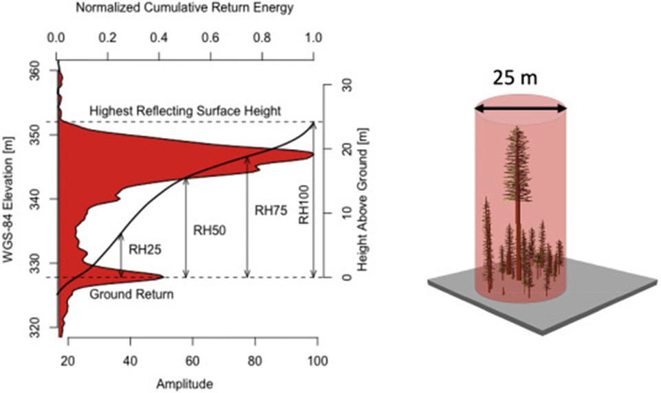
2.3. Lidar remote sensing

Lidar¹ measurements can be used to estimate tree height with good accuracy. This measurement is usually combined with other remote sensing measurements (see above) to estimate forest biomass. The advantage of this method is that it allows for fairly accurate estimates, whether at the regional level (measurements from an aircraft) or the global level (satellite measurements). However, measurements can become saturated and estimates made by lidar are generally static, as it takes several years to cover the entire globe by satellite measurements. Example: NASA / GEDI satellite (Figure 1) [5].

2.4. Microwave remote sensing

These observations are made with instruments that measure the natural emission (passive domain) or the backscatter (active or radar domain) of plant cover in the microwave domain. These measurements allow us to estimate the attenuation effect of microwave radiation by the vegetation cover. This attenuation (associated with the Vegetation Optical Depth, VOD) is well related to the biomass of the vegetation. Compared to optical measurements, microwave measurements are little affected by cloud cover and atmospheric effects and saturate less quickly at high forest vegetation densities. Depending on the used methods (passive or active instruments) and wavelengths, the obtained spatial resolution (from a few meters to several kilometers) and the saturation threshold are variable.

3. The Biomass Carbon Monitor project

On October 29, 2021, the Biomass Carbon Monitor the first geospatial platform capable of measuring the role of forests in carbon sequestration by observing changes in biomass was published. Kayrros [6], in partnership with the French National Research Institute for Agriculture, Food and the Environment (INRAE) and the French Laboratory for Climate and Environmental Sciences (LSCE), developed this tool based on 30 years of research. It is now freely available to all.

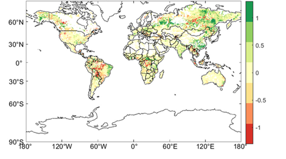
The Biomass Carbon Monitor provides free access to global maps of changes in carbon stocks contained in aboveground biomass. The data allow quantifying annual changes in biomass and determining the role that forests play in reducing the amount of carbon in the atmosphere.

The Biomass Carbon Monitor data are derived from systematic measurements of microwave emission from land surfaces by the European SpaceAgency‘s (ESA) SMOS satellite, combined with particularly advanced algorithms. The result shows that some regions of the northern hemisphere store carbon, while tropical regions affected by deforestation are emitters. Globally, 760 million tons of carbon (Mt) have been removed from the atmosphere each year over the past decade [7] – offsetting nearly 8% of the CO₂ emissions associated with fossil fuel consumption and cement production during that time.

---

Notes and references

Cover image.

[1] Baccini, A. et al. Tropical forests are a net carbon source based on aboveground measurements of gain and loss. Science 358, 230-234 (2017), https://doi.org/10.1126/science.aam5962

[2] Chave, J. et al. Improved allometric models to estimate the aboveground biomass of tropical trees. Glob. Chang. Biol. 20, 3177-3190 (2014).

[3] Hansen, M. C. et al. High-resolution global maps of21st-century forest cover change. Science 342, 850-853 (2013). https://doi.org/10.1126/science.1244693

[4] Harris, N.L., Gibbs, D.A., Baccini, A. et al. Global maps of twenty-first century forest carbon fluxes. Nat. Clim. Chang. 11, 234-240 (2021). https://doi.org/10.1038/s41558-020-00976-6

[5] Dubayah, R. et al. The Global Ecosystem Dynamics Investigation: high-resolution laser ranging of the Earth’s forests and topography. Sci. Remote Sens. 1, 100002 (2020), https://doi.org/10.1016/j.srs.2020.100002

[6] Boutaud, A.-S. Kayrros, le big data au service de la transition écologique. CNRS, le journal(15.06.2022). https://lejournal.cnrs.fr/nos-blogs/de-la-decouverte-a-linnovation/kayrros-le-big-data-au-service-de-la-transition-ecologique

[7] This value of 0.76 GtC/year estimated by the Biomass Carbon Monitor project for the carbon sink due to continental photosynthesis is lower than the 1.8 GtC/year of the Global Carbon Project (see Figure 2). This again shows that there are many uncertainties in the absolute values of forest carbon fluxes and stocks.