It is impossible to weigh every organism on the planet. Researchers therefore combine local measurements, conversions to carbon mass, environmental maps and extrapolation models. They do not obtain an exact figure, but rather an order of magnitude accompanied by a margin of uncertainty. Remote sensing, automated imaging and molecular analyses extend the coverage of observations, without eliminating biases associated with regions and organisms that are sparsely sampled.

1. A common unit for comparing living organisms

Biomass refers to the mass of living organisms present at a given time. It can be expressed as fresh mass, dry mass or carbon mass. To compare a tree, a bacterium and a fish, global summaries generally use the gigatonne of carbon (Gt C; 1 Gt C = 10¹⁵ g of carbon). This unit prevents differences in water content from skewing comparisons. It provides no information on the number of species or individuals, nor on annual production (see the focus section on Species, individuals and biomass).

A biomass estimate describes a carbon stock at a given point in time, rather than a flux such as annual primary production. Thus, phytoplankton forms a small, rapidly renewed stock, whilst trees accumulate significant biomass over decades (see ‘Phytoplankton: a small stock, immense production’).

The scope must be clearly defined. Estimates relate to living matter and generally exclude dead wood, litter, soil organic matter and dissolved organic carbon. Viruses are sometimes estimated separately, as whether they are living organisms remains a matter of debate. Parasites, symbionts and microbiota must be treated with care to avoid double counting.

2. From local samples to global estimates

The review published in 2018 by Bar-On et al. [1] remains the most comprehensive reference for comparing the biomass of the major groups of living organisms. Their approach comprises four stages (Figure 1).

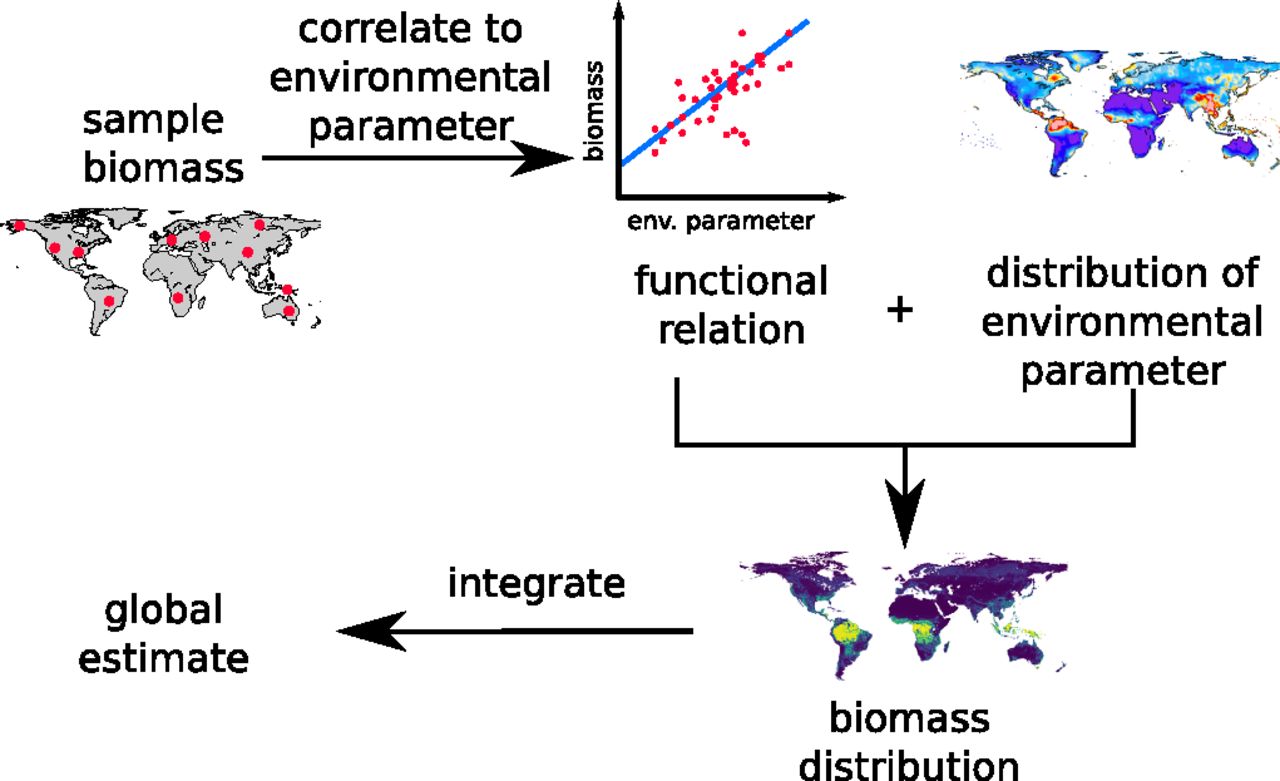
1. Measure locally and convert to carbon. At sites that are as representative as possible, researchers collect or observe organisms, then measure mass, abundance, volume, surface area or concentration. Carbon mass is measured directly or calculated using a conversion factor: average mass, size-mass relationship, cellular biovolume, carbon content of dry matter or an allometric equation.
2. Link observations to the environment. Local densities are correlated with variables available on a large scale: climate, depth, soil type, vegetation, productivity, distance from the coast or forest structure.
3. Extrapolate. A model estimates biomass density in unsampled regions, at a resolution that depends on that of the environmental variables.
4. Integrate. Densities are summed over the entire area or volume occupied. The convergence of independent methods enhances the robustness of the result.

Two approaches complement each other:

• The bottom-up approach extrapolates densities obtained from measurements taken on organisms, samples or plots.
• The top-down approach utilises large-scale observations, such as satellite data, calibrated against local measurements.

The most robust estimates compare methods whose errors are not entirely shared. Uncertainty accumulates at each stage: sampling, counting, carbon-conversion and spatial extrapolation. The uncertainty of the global total therefore does not depend solely on the final model.

When positive estimates differ mainly by multiplicative factors, their geometric mean, calculated on a logarithmic scale, limits the influence of an exceptionally high value.

3. Methods tailored to organisms and environments

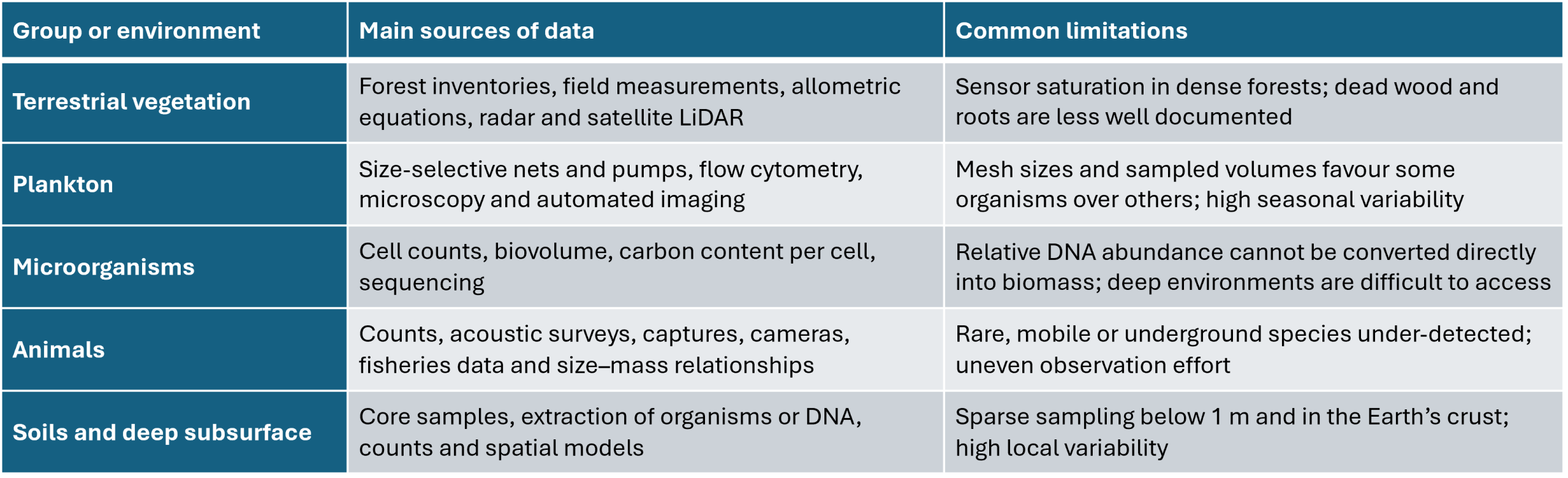
No single method can estimate the biomass of all living organisms. The strategy depends on the size of the organisms, their habitat, their mobility and their detectability (Table 1). Recent techniques extend the coverage of observations, but they only provide a biomass estimate after calibration using direct measurements.

Table 1. Main data used to estimate the biomass of different groups or environments, and limitations frequently encountered. As no single method allows for a comprehensive inventory, global estimates combine field observations, remote sensing, biological analyses and models.

3.1. Terrestrial plants: inventories, allometry and remote sensing

The forest inventories compiled by the FAO from national reports [2] measure, in particular, the diameter and height of tree trunks, and sometimes wood density. Allometric equations are used to derive above-ground biomass from these measurements. Roots, which are rarely measured, are generally estimated based on the ratio of below-ground to above-ground biomass.

These local observations are used to calibrate remote-sensing maps [3]. Satellite instruments do not directly weigh trees: radar and LiDAR describe the height, density and structure of the canopy, and measurements taken on sample plots then link these signals to biomass.

Since 2019, the GEDI mission has been providing LiDAR profiles of vegetation [4]. When combined with other satellite imagery, they improve aerial biomass maps but provide less accurate information on roots and very dense forests. Launched in April 2025, the Biomass mission of the European Space Agency (ESA) uses the first P-band orbital radar. Its long wavelengths penetrate the canopy and enable better characterisation of woody biomass. The data have been freely available since early 2026; derived products are being announced/scheduled for release progressively for 2026-2027 [5].

3.2. Plankton and other marine organisms

Marine organisms are collected using nets, pumps or bottles suited to their size (Figure 2). Microscopy, cytometry and imaging provide counts, sizes or biovolumes. These measurements are converted into carbon and then extrapolated to the water column and region under study.

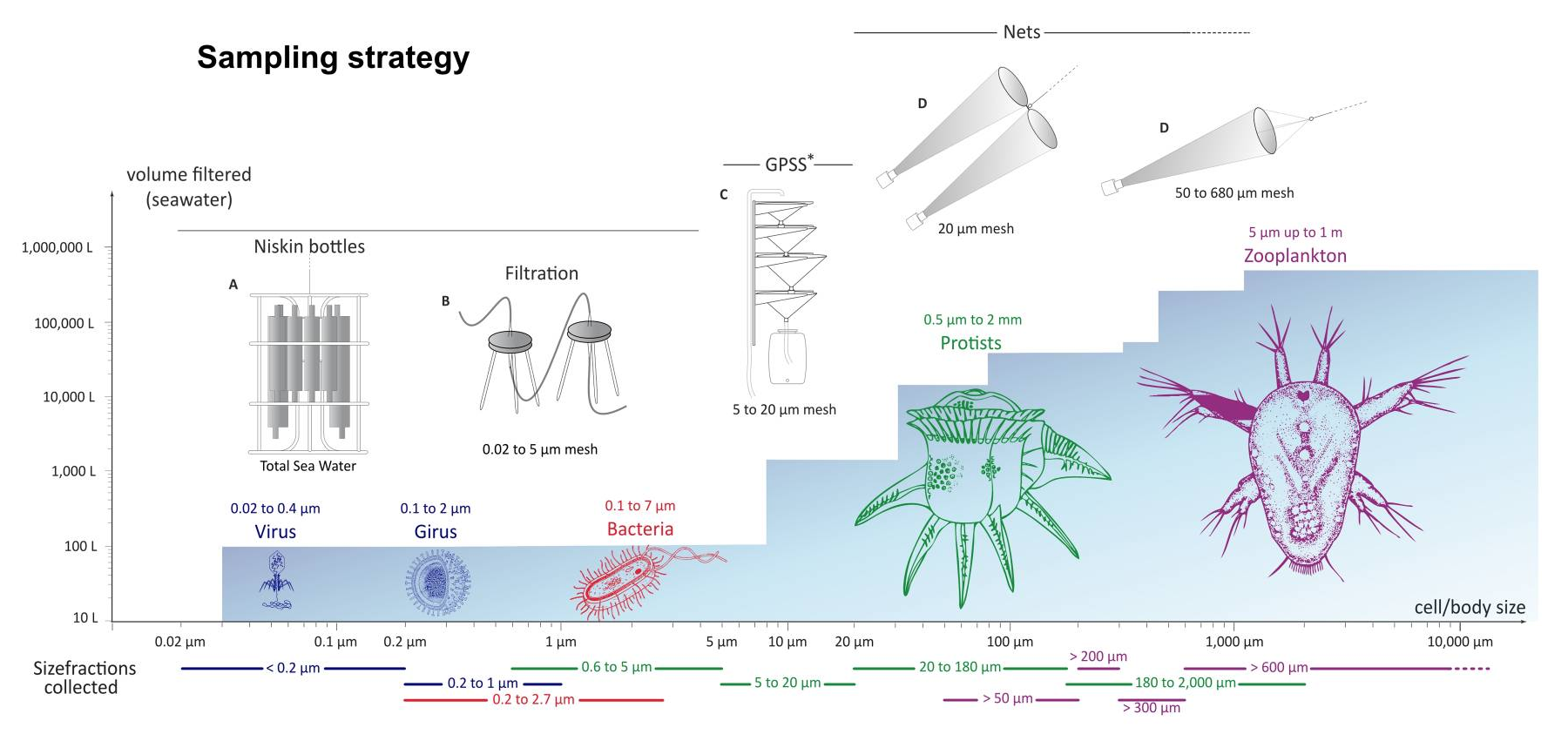
No single method covers viruses, phytoplankton, zooplankton and large animals [6],[7]. Campaigns such as Tara Oceans therefore combine several sampling techniques. Flow cytometry and automated imaging enable the analysis of large numbers of organisms, whilst algorithms facilitate their classification. The scope of observations is expanding, but instrument calibration and taxonomic validation remain essential.

3.3. Microorganisms in soil, sediments and the subsoil

In known volumes of soil, sediment or rock, the number of cells is estimated using microscopy, cytometry or molecular markers. This is then converted into carbon and extrapolated to the volume of the medium. The depth studied, the heterogeneity of habitats and the distinction between living and dead cells strongly influence the result [8].

Environmental DNA also makes it possible to detect organisms in water, soil or sediments that are difficult to observe. It thus improves diversity inventories and the detection of rare organisms. However, the number of sequences depends on the number of gene copies as well as on DNA extraction and preservation methods. It therefore cannot be directly converted into the number of individuals or biomass. A meta-analysis concludes that this relationship is weak and highly uncertain [9]. Molecular data complement physical measurements without replacing them.

3.4. Animals: population numbers multiplied by average body mass

For humans, farmed animals or certain wild vertebrates, recorded or estimated population numbers are combined with an average body mass and carbon content. Age structure, differences in size and gaps in inventories remain sources of uncertainty.

This approach has also been applied to groups that are difficult to survey on a global scale, such as soil nematodes, ants and wild mammals [10].

4. Estimates to be interpreted with caution

4.1. The main sources of uncertainty

• Spatial bias. Easily accessible sites are over-represented, whilst the deep sea, deep soil layers, polar regions and certain tropical regions remain under-sampled. Neglecting these habitats leads to an underestimation of biomass; conversely, relying primarily on sites that are very rich in organisms tends to lead to an overestimation.
• Temporal bias. A one-off survey may fail to capture seasonal variations, migrations, population booms or rapid changes linked to human activities.
• Detection bias. Organisms that are very small, rare, mobile, fragile or attached to a substrate are more likely to escape sampling devices.
• Conversion uncertainty. An average mass or a relationship between size and mass does not perfectly represent individuals that differ in age, physiological condition and species.
• Model uncertainty. A relationship observed in some regions may not hold true elsewhere. The environmental maps used themselves have limited resolution and contain errors.
• Taxonomic gaps and double counting. Certain practical categories, such as protists, encompass very different lineages. Parasites, symbionts and microbiota may be overlooked, misidentified or counted alongside their hosts.

4.2. How to express and interpret uncertainty

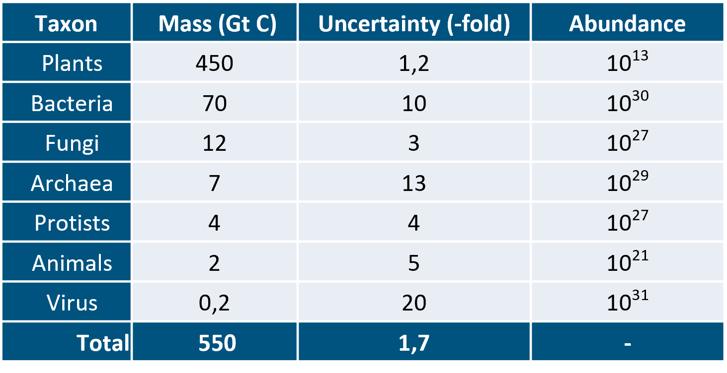
Global uncertainties are often multiplicative. Thus, an estimate of 70 Gt C accompanied by a factor of 10 corresponds approximately to a range of 7 to 700 Gt C. Bar-On et al. present these ranges as the equivalent of a 95 per cent confidence interval [1]. However, they combine calculations based on data and, where data are lacking, comparisons with analogous groups and expert opinions. They therefore describe plausible values, without always constituting statistical intervals established from independent samples. Table 2 summarises the results of Bar-On et al. by kingdom. This classification, which is now open to debate, corresponds to the taxonomic resolution of the available data. Viruses are estimated separately, whilst animal biomass is calculated by summing the main phyla [1].

Table 2. Estimated total biomass of the main taxonomic groups. The values, derived from a review of the literature, are rounded to account for their uncertainty; the sum of the detailed rows may therefore differ from a group’s total. Uncertainty is expressed as a multiplicative factor: it is high for bacteria (7 to 700 Gt C), but much lower for plants (approximately 375 to 540 Gt C). [According to Bar-On et al. [1]; CC BY-NC-ND 4.0 licence]

Plant biomass is the best constrained (factor 1.2), thanks to the FAO’s forest inventories [2] and remote sensing [3]. For bacteria, archaea and viruses, uncertainties reach a factor of 10 to 20, notably due to a lack of data on the deep subsurface. Viruses — particularly bacteriophages and archaeal viruses — illustrate this difficulty: the parameters required for their estimation remain scarce [1].

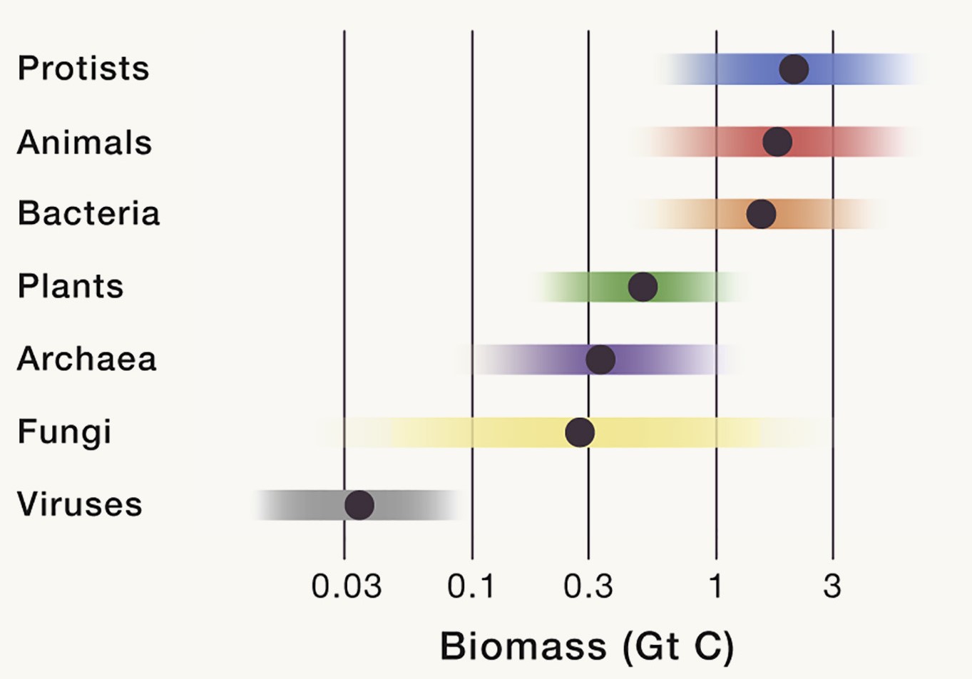
Marine prokaryotes illustrate how these uncertainties are calculated (Figure 3). Cell concentrations are grouped by depth, multiplied by the corresponding volume of water, and then converted to carbon using an average content per cell [10]. For less well-studied groups, such as arthropods or terrestrial protists, the risk of systematic bias is higher.

A distinction must be made between natural variability, sampling error, conversion or modelling uncertainties, and unquantified biases. Increasing the number of samples reduces sampling error but does not correct for the absence of a habitat in the data or an incorrect conversion factor. A seemingly precise value may therefore still be inaccurate.

4.3. Regularly revised estimates

The 2018 survey provides consistent orders of magnitude, rather than a simultaneous and definitive measurement of the biosphere: its data are drawn from different years, regions and methods. Since then, inventories have refined estimates of the biomass of soil nematodes, ants and wild mammals [10]. A global compilation thus estimates the biomass of prokaryotes in the continental subsoil at 23–31 Gt C, which is 4 to 10 times less than previous values [8]. This total, including archaea, remains lower than the 70 Gt C attributed to bacteria alone, but falls within their uncertainty range of 7 to 700 Gt C. It demonstrates the extent to which coverage of deep environments influences global estimates.

Each figure must therefore be considered in the context of its date, methodology, scope and uncertainty. A revision does not necessarily reflect an actual change: it may result from improved coverage, a new conversion factor or a more accurate model. Tracking trends requires repeated and comparable observations, obtained using a consistent protocol.

5. Messages to remember

• Global biomass is estimated by combining local measurements, carbon conversions and spatial extrapolations.
• Carbon mass allows for the comparison of organisms that differ significantly in water content and size.
• Each group of living organisms requires a tailored method; no single technique covers the entire biosphere on its own.
• Satellites, automated imaging and environmental DNA improve observations, but do not replace measurements taken on land or at sea.
• Any global estimate must be interpreted in the context of its range of uncertainty, its date and its main sources of bias.
  

  ---

  Notes & references

  Thumbnail. Photo via Pixabay

  The reviews by Bar-On et al. (2018), Bar-On and Milo (2019) and Greenspoon et al. (2023) serve as the references for the distribution figures presented here. The articles are published as ‘open access’ and distributed under a Creative Commons licence.

• Bar-On Y.M., Phillips R. & Milo R. (2018) The biomass distribution on Earth. Proc. Nat. Acad. Sci. U.S.A. 115:6506-6511; https://www.pnas.org/doi/10.1073/pnas.1711842115. The data has been deposited to GitLab (https://github.com/milo-lab/biomass_distribution).
• Bar-On Y.M. & Milo R. (2019) The biomass composition of the oceans: A blueprint of our blue planet, Cell, 179 :1451–1454; https://doi.org/10.1016/j.cell.2019.11.018. The data has been deposited to GitLab (github.com/milo-lab/ocean_biomass)
• Greenspoon L., Krieger E., Sender R., Rosenberg Y., Bar-On Y.M., Moran U., Antman T., Meiri S., Roll U., Noor E., & Milo R. (2023), The global biomass of wild mammals, Proc. Natl. Acad. Sci. U.S.A. 120 (10) e2204892120, https://doi.org/10.1073/pnas.2204892120. The data has been deposited to GitLab (https://gitlab.com/milo-lab-public/mammal_biomass/)

 

[1] Bar-On Y.M., Phillips R. & Milo R. (2018). The biomass distribution on Earth. Proceedings of the National Academy of Sciences, 115, 6506–6511. https://doi.org/10.1073/pnas.1711842115

[2] MacDicken K.G. (2015). Global Forest Resources Assessment 2015: What, why and how? Forest Ecology and Management, 352, 3–8.

[3] Saatchi S.S. et al. (2011). Benchmark map of forest carbon stocks in tropical regions across three continents. Proceedings of the National Academy of Sciences, 108, 9899–9904. https://doi.org/10.1073/pnas.1019576108 – Baccini A. et al. (2012). Estimated carbon dioxide emissions from tropical deforestation improved by carbon-density maps. Nature Climate Change, 2, 182–185 – Thurner M. & Beer C. (2014). Carbon stock and density of northern boreal and temperate forests. Global Ecology and Biogeography, 23, 297–310.

[4] Dubayah R. et al. (2020). The Global Ecosystem Dynamics Investigation: High-resolution laser ranging of the Earth’s forests and topography. Science of Remote Sensing, 1, 100002. https://doi.org/10.1016/j.srs.2020.100002

[5] ESA (2026). ESA’s Biomass goes live with data now open to all. 26 janvier 2026. https://www.esa.int/Applications/Observing_the_Earth/FutureEO/Biomass/ESA_s_Biomass_goes_live_with_data_now_open_to_all – ESA Earth Online (2026). Biomass Level-2 product release schedule. 26 mars 2026. https://earth.esa.int/eogateway/news/biomass-level-2-product-release-schedule

[6] Bar-On Y.M. & Milo R. (2019). The biomass composition of the oceans: A blueprint of our blue planet. Cell, 179, 1451–1454. https://doi.org/10.1016/j.cell.2019.11.018

[7] de Vargas C. et al. (2015). Eukaryotic plankton diversity in the sunlit ocean. Science, 348, 1261605. https://doi.org/10.1126/science.1261605

[8] Magnabosco C. et al. (2018). The biomass and biodiversity of the continental subsurface. Nature Geoscience, 11, 707–717. https://doi.org/10.1038/s41561-018-0221-6

[9] Lamb P.D. et al. (2019). How quantitative is metabarcoding: A meta-analytical approach. Molecular Ecology, 28, 420–430. https://doi.org/10.1111/mec.14920

[10] van den Hoogen J. et al. (2019). Soil nematode abundance and functional group composition at a global scale. Nature, 572, 194–198. https://doi.org/10.1038/s41586-019-1418-6 – Schultheiss P. et al. (2022). The abundance, biomass, and distribution of ants on Earth. Proceedings of the National Academy of Sciences, USA, 119, e2201550119. https://doi.org/10.1073/pnas.2201550119 – Greenspoon L. et al. (2023). The global biomass of wild mammals. Proceedings of the National Academy of Sciences, USA, 120, e2204892120. https://doi.org/10.1073/pnas.2204892120