


遗传多态性和选择
多态性在进化中扮演的角色引起了争论。但是如果多态性本质上是一种中性进化,那么它反过来就可以作为研究自然选择的参照。生态学家在保护生物学中也利用它来重建物种过去的历史。
1. 突变,随机漂变和中性进化
多态性包括在细胞分裂时逃脱了DNA修复系统的突变,因此突变率是一个生物学变量。在人类和黑猩猩中,每一世代核苷酸核酸(如DNA或RNA)的组成单元。它由一个核碱基(或含氮碱基)、一个称为戊糖的五碳糖组成,它们结合形成核苷,然后与一到三个磷酸基团相连接。的突变率约为μ≈10-8。雄性哺乳动物产生大量的精子,这意味着雄性种系从干细胞到配子的所有细胞。比雌性种系更多:30岁时比例是380:23(即16倍以上),并且随着雄性的年龄增长比例会更高(50岁时是840:23,即36倍以上)。这意味着,在这些物种中突变主要在雄性系中产生,且取决于父亲的年龄。每次生殖都会在基因组生物体的遗传物质。它包含编码蛋白质的遗传信息。在大多数生物体中,基因组对应于DNA。然而,在一些称为逆转录病毒的病毒(例如HIV)中,遗传物质是RNA。中产生约100个新的突变,但因为基因组中只有很小一部分是编码描述基因的DNA或RNA中被翻译成蛋白质的部分。仅代表其起源的基因的一部分,以及其内嵌的mRNA。的,所以99%的突变不影响生存和繁殖能力。这些突变称为中性突变。一个新的等位基因如果两个同源基因具有不同的形式,并且在特定的观察水平上可以区分,那么这两个基因就是等位基因。因此,等位基因可能对应于一个序列,也可能对应于一组在表型水平上无法区分的不同序列。(例如,蓝色/棕色/绿色的眼睛颜色,但在核苷酸水平上有更多不同的等位基因,每种颜色有几种)。可以是中性的、有害的或者是有益的。中性突变是研究最多的变异,因为它们可以用来编写预测模型,研究种群的历史。中性突变的分布也可以作为一个零假设指基本观点,即对某一现象的默认立场。一般来说,反对零假设的假设有举证责任。,通过比较来解释有害或有益突变的分布。
我们可能会认为,在一个只包含中性等位基因的基因组中,等位基因频率的漂移会在一次又一次的波动中自我补偿,等位基因多样性H会长期保持稳定。但这种印象是错误的。多样性会逐渐遭到侵蚀,这与人类社会中姓氏多样性的丧失非常相似,虽然它确实是一种缓慢的现象,但在偏远农村等与世隔绝的地方却很明显。当一个家庭没有儿子时,姓氏就无法传递。虽然该姓氏可以由亲戚家庭传承下去,但随着这个家族人口减少,该姓氏消亡的可能性就会增大。这显然与男孩出生时携带Y染色体的任何生物学特性无关。概率就足以解释这一点。这一特性反映了一个事实,即亲代群体的子代遵循重置抽样从一个装有n个令牌的瓮中连续有回放地抽取p个令牌。即抽取第一个令牌后记录它的值,然后把它放回瓮中;再抽取第二个令牌,记录它的值后又放回瓮中,依次进行,直到抽取第p个令牌为止。这相当于从n个对象中选择p个对象,而且是可重复选择(可以多次选择同一个对象)和有顺序选择(选择对象的顺序很重要)。从n中连续抽取p个对象的可能性组合数为:n×n×n×…×n=np。的原则。
与 Y 染色体一样,亲代的一些基因没有被抽出,在子代群体中也找不到。如果子代的基因是从一个大小不变的群体中随机抽取的,那么未被抽取的基因的概率由参数为 1 的泊松分布给出,即q(0) = e-1 = 0.367。这些未被提取的基因(超过三分之一)在没有后代的情况下就丧失了。亲代基因如果偶然留下更多的后代,就可能弥补一部分损失。如果没有完全补偿,那么溯祖谱系就会保持平行而不会有交点。我们向前溯祖时的谱系组合过程与我们向后直到当前的检视过程中多样性的丧失没有什么不同,也与所谓的近亲繁殖没有什么不同。
公式(1)中的多样性度量有一个有用的特性:它取决于估算样本的大小。根据公式E(Hs) = Ht (1 – 1/n),当从”t”亲代中抽取n个基因作为”t+1″子代种群的样本时,子代的变异损失等于1/n。因为是随机抽取,所以即使子代种群大于亲代种群,情况也是如此;但是种群越大,多样性受到的侵蚀就越小。上式成立的条件是种群规模有限,而所有真实的种群都是如此。按照惯例,遗传学家将这种变异损失记作1/Ne,其中Ne是染色体的有效数目[1]。因此从第一代到第二代:
E(H2) = H1 (1 – 1/Ne) (3)
有效数目几乎总是比染色体的实际数目少得多,原因将在后面讨论。例如,据估计,在人类过去的谱系中,有效染色体数量大约为10,000 条。如果没有变异,那么经过一段时间T(期望)后将变成单态:
E(T) = 2 Ne (4)
这将导致两个结果:首先,一个物种的多态性在该物种的持续时间范围内总是“最近期的”。这是因为多态性依赖于突变,尽管伴随着等位基因频率的漂移多样性遭到侵蚀,而突变能恢复多态性。其次,多态性水平是两种对立机制的权衡,形成了中性突变–漂移平衡。
多态性随着时间的推移而消失可以用相反的方式来表示:当我们追溯到过去,在同一基因位点基因在染色体上的位置。在群体遗传学中,指一组同源基因(同源类)。如果两条染色体或两个基因在减数分裂过程中相互匹配并相互排斥,那么这两条染色体或两个基因就是同源的。上的两个基因之间总有一个最后的共同祖先。这就是约翰-金曼所说的(John Kingman)所说的溯祖过程。不同位点的祖先并不相同,因为有性过程使祖先的数量成倍增加,因此也使基因的共同祖先成倍增加。如果上一代有共同祖先的概率q = 1/Ne随时间保持不变,那么祖先的分布就会遵循指数变化规律t = q.e-qt。这些祖先的预期年龄为Ne。如果从那时起没有发生变异,那么两个基因在遗传上将是相似的。但是,只要从祖先到两个基因中的每一个基因的其中一条线上发生了突变,这两个基因就会成为等位基因。由此我们可以推断,这两个基因之间的核苷酸差异数等于θ = Ne x 2µ,其中µ是中性突变率。这个定义为θ = 2Neµ 的值θ是群体遗传学中的一个基本参数。
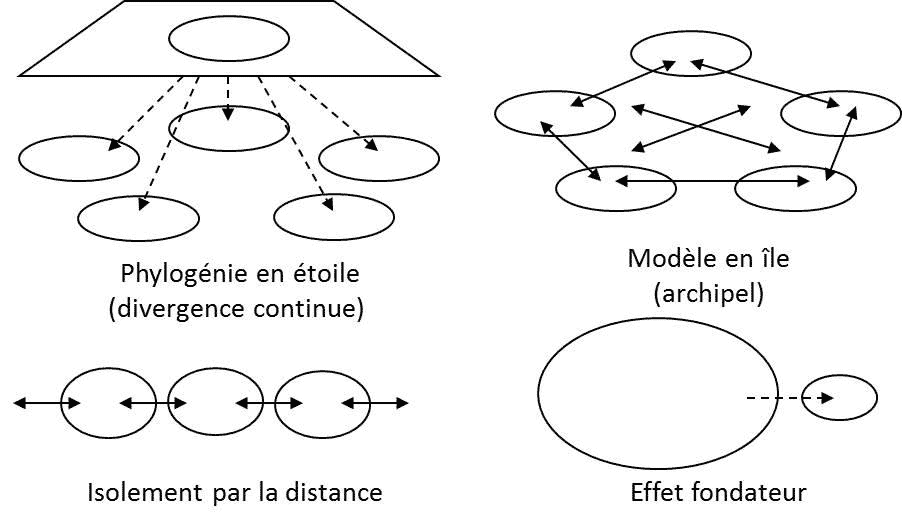
自然种群的中性进化在保护生物学中非常重要,因为这能帮助重建物种的历史。遗传学家早就知道,随机遗传漂变能帮助构建种群分化和物种空间分布的模型(图1)。在20世纪下半叶,研究亚种群组成种群的最常用的指标是FST,其公式为:
FST = 1-HS/HT (5)
其中HS为各亚种群多样性的平均值,HT为种群多样性[2]。
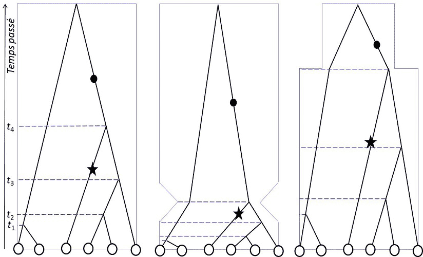
在数字基因组分析时代的21世纪,金曼(Kingman)、哈德逊(Hudson)和田岛(Tajima)在1982-83年独立提出了溯祖理论[3],除了用于研究种群结构,还能确定种群是否保持了稳定或发生了种群统计学上的变化(图2)。
2. 中性模型和生物多样性管理
图1和图2说明了遗传变异模式受种群历史影响的程度:空间结构、定殖、迁移和种群规模的变化都会在物种的分子多态性上留下特定的印记,使生态学家能够追溯种群的历史。在第四纪(也就是现在的地质时期)地球的气候发生了周期性变化,导致海岸线周期性变化、生物群落和冰川南北移动,导致各纬度都出现了潮湿或干燥气候旋回。种群生物学家在采取任何自然种群管理的举措之前,都会系统地记录由此产生的种群迁移、减少、增加和入侵情况,这些都是物种响应环境变化的指标。目前,种群遗传学主要应用于保护生物学领域。
3. 有害突变
由于基因编码蛋白质,编码区的大多数突变都会改变蛋白质序列(约占突变的3/4,这一比例随序列的组成而变化)。在人类谱系中,这些变化中约有40%是有害的,也就是说,当我们对人类从黑猩猩谱系分离出来后的基因组进化进行评估时,我们观察不到这些变化。如果一个突变是中性的,那么它有一天取代该位点上其他基因的几率为1/Ne(在一个有效大小为Ne的种群中,其他基因加在一起的比例为1-1/Ne,每个基因取代所有其他基因的几率也是1/Ne)。但突变可能是有害的,会影响携带突变个体的健康或繁殖能力。突变的频率会在随机漂移的作用下波动几代,然后在选择作用下消失(在果蝇中的存在时间平均为40代)。一个物种的所有成员都是有害突变的携带者,你我都是。有害突变几乎总是处于杂合状态,因为如果一个突变的频率是1/1000,那么呈纯合子指生物体的每条同源染色体上的同一基因座上都有两个相同的等位基因。的突变比杂合子指生物体的同源染色体上的同一基因在同一位点上有两个不同的等位基因。低一千倍。正是杂合子的轻微劣势清除了突变,而不是纯合子往往大得多的劣势。由于几个基因位点上的有害突变的影响是累积性的,突变负荷表现为一个数量变量,其加性效应可能无法检测到,但却能长期有效地把有害突变从基因组中清除掉。这就解释了为什么蛋白质仍然具有功能,为什么有害突变的频率仍然很低。这无疑是基因重组得以维持的原因之一。基因重组使有害突变可以集中起来,并消除它们,同时还能控制清除有害突变对染色体相邻区域的影响。
4. 有利突变
在影响蛋白质的突变中,有 60%不会产生有害效应。与影响基因组其他区域的突变一样,它们可能是”中性”的,即在特定环境和特定物种中对健康或繁殖能力没有任何影响。它们的频率在自然种群中随机波动。但如果条件发生变化,它们也可能变得有利。这就是达尔文(Darwin)所设想的自然选择和性选择的结果,也是选择一词最初的含义,即人类对其驯化物种的选择。被选择的多态性有两种类型:瞬时多态性和平衡多态性。
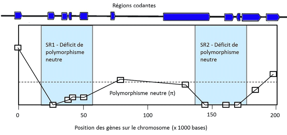
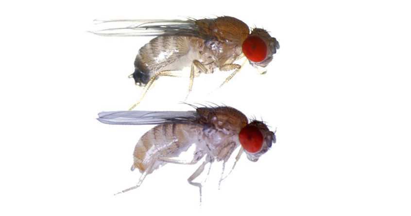
瞬时多态性是指一个有利突变通过清除其他等位基因而逐渐自我“固定”下来的过程,这可能导致该基因的频率为1。例如,蚊子的杀虫剂抗性基因、细菌的抗生素抗性基因和导致疟疾的寄生虫的抗疟药物抗性基因。在自然条件下,这些突变基因可能没有任何优势,但在使用药物的情况下,这些等位基因的频率就会增加。调节乳糖酶表达的三个等位基因也是这种情况,乳糖酶使人类不仅能像其他哺乳动物一样在刚出生时消化乳糖,而且在成年后也能消化乳糖。这些突变在从事畜牧业的人群中变得有益,而我们狩猎采集的祖先只有在成年后才有机会消化果糖(蔗糖)。在所有这些瞬时多态性的案例中,选择所作用的位点被基因组中的一个特征”出卖”了:该位点基因频率的迅速增大导致染色体上相邻的中性变异消失。这是一种选择性清除(selective sweep)的情况,意味着等位基因的固定不是由于随机漂移,而是由于选择作用(图3,[4])。
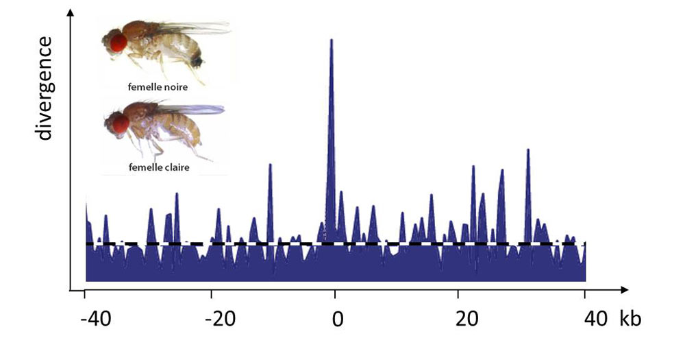
平衡多态性是指两个等位基因共存的情况,因为每个等位基因都只在某些条件下具有优势,但任何一个等位基因都不是在所有时间或空间条件下优于另一个等位基因。基因型的选择优势与其频率成反比就是一个例子,这就是所谓的频率依赖性选择。性选择经常出现这种平衡多态性(图4,[5])。
5. 多态性有用吗?
从20世纪30年代到60年代,群体遗传学家在自然界中发现了越来越多的多态性。他们希望评估这些多态性的程度,并探究它们在进化方面的潜在用途。有人认为,遗传多样性本身就具有优势,而选择使其保持在较高水平;也有人认为,选择导致野生种群产生了相当单一的表型个体的所有可观察到的特征。,而与此不同的变异则相当有害。他们的观点都不正确。20世纪50年代,法国人古斯塔夫-马勒科(Gustave Malécot)证明,中性多态性是孟德尔定律捷克僧侣、植物学家格里高尔-孟德尔(1822-1884 年)提出的有关生物遗传原理的定律。在有限种群中的结果[6]。最后,日本科学家木村(Kimura)和太田(Ohta)于1966年发现了极高的分子多态性水平,而这种多态性无法仅用自然选择来解释[7],从而提出了中性理论[8]。人们意识到,达尔文自然选择理论的替代方案并不是物种的固定性(这是达尔文的反对者所持观点),而是中性模型所预测的持续遗传变化,类似于物理学中扩散现象的无规行走(random walk)。这一观点最终在20世纪80年代被接受。然而,与繁殖种群的规模相比,在所有物种中测得的有效种群规模的数值都非常低,这表明各种力量对遗传多样性的侵蚀远远超过了中性模型的预测。这种侵蚀有一部分是自然选择的结果,它消除了有害的变异并固定了有利的变异,从而增加了漂移对中性变异的影响。尽管选择性多态性对物种的未来极为重要,但它肯定只占多态性的极小一部分。
中性分子多态性提供了研究选择和种群历史的基本理论和参考模型。矛盾之处在于,现在人们正在利用中性理论在基因组中寻找自然选择的分子特征。
使重组系统、孟德尔定律(Mendel’s laws)[9],以及通过有性繁殖进行基因混合得以维持的选择性力量的存在,证明在自然种群中多态性维持在短期是有益的。
参考资料及说明
[1] 直到 2000 年左右,有效个体数都是以个体而不是以染色体来表示的,因此,在繁殖过程中雌雄个体数相同的情况下,常染色体的有效个体数为2Ne,X染色体为1.5Ne,Y染色体和线粒体为0.5Ne。这些公式可以在教科书中找到。
[2] 这个公式在这里是非常笼统的,根据所使用的遗传模型,它有多种形式和名称:Wright的FST(两个等位基因)、Nei的GST(FST的推广,上面公式5的变体)、ΦST、ρST等等。它可以被类似性质的统计数据所替代:DXY、AMOVA。这种冗余首先表明了“F统计量”在生态学中的成功。由于估计值依赖于样本量,使用无偏估计值时,也必须考虑到观测设计的特殊性。参见: Weir B.S. & Cockerham C.C. (1984) Estimating F-statistics for the analysis of population structure. Evolution 38:1358-1370
[3] Kingman J.F.C. (1982) On the genealogy of large populations. Journal of Applied Probability 19A:27-43; Hudson R.R. (1983) Properties of a neutral allele model with intragenic recombination. Theoretical Population Biology 23:183-201; Tajima F. (1983) Evolutionary relationship of DNA sequences in finite populations. Genetics 105:437-460.
[4] Derome N., K. Métayer, C. Montchamp-Moreau & M. Veuille (2004) Signature of selective sweep associated with the evolution of sex-ratio drive in Drosophila simulans. Genetics 166: 1357-1366; Derome N., E. Baudry, D. Ogereau, M. Veuille & C. Montchamp-Moreau (2008) Selective sweeps reveal a two-locus model for sex-ratio meiotic drive in Drosophila simulans. Molecular Biology and Evolution, 25:409-416.
[5] Yassin A., Bastide H., Chung H., Veuille M., David J.R. & Pool J.E. (2016) Ancient Balancing Selection at tan Underlies Female Colour Dimorphism in Drosophila erecta. Nature Communications DOI: 10.1038/ncomms10400.
[6] Malecot G. (1948) The mathematics of heredity. Masson et Cie; Nagylaki T. (1989) Gustave Malécot and the transition from classical to modern population genetics. Genetics 122, 253-268.
[7] Lewontin R.C. & Hubby J.L. (1966) Molecular Approach to the Study of Genic Heterozygosity in Natural Populations. II. Amount of Variation and Degree of Heterozygosity in Natural Populations of Drosophila pseudoobscura, Genetics 54: 595-609; Lewontin R.C. (1974) The Genetic Basis of Evolutionary Change. Columbia Univ. Press, New York.
[8] Kimura M. (1969) The Rate of Molecular Evolution Considered from the Standpoint of Population Genetics. Proceedings of the National Academy of Sciences, 63:1181-1188.
[9] http://uel.unisciel.fr/biologie/analgen/analgen_ch01/co/learn_ch1_01_01_01.html
环境百科全书由环境和能源百科全书协会出版 (www.a3e.fr),该协会与格勒诺布尔阿尔卑斯大学和格勒诺布尔INP有合同关系,并由法国科学院赞助。
引用这篇文章: VEUILLE Michel (2024年10月18日), 遗传多态性和选择, 环境百科全书,咨询于 2026年7月29日 [在线ISSN 2555-0950]网址: https://www.encyclopedie-environnement.org/zh/vivant-zh/genetic-polymorphism-and-selection-2/.
环境百科全书中的文章是根据知识共享BY-NC-SA许可条款提供的,该许可授权复制的条件是:引用来源,不作商业使用,共享相同的初始条件,并且在每次重复使用或分发时复制知识共享BY-NC-SA许可声明。