


Astronomical theories of climate: a long history
PDF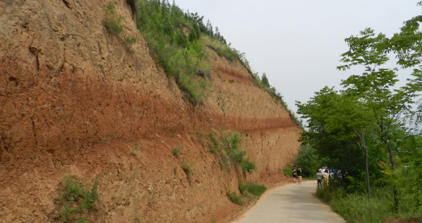
What have been the characteristic periods of climatic variations over the last few million years? Those responsible for these natural variations are the parameters of the Earth’s movement around the Sun: eccentricity of its elliptical trajectory, obliquity and precession of its axis of rotation. How did the astronomers of the 18th century get the intuition of alternating glaciations and interglacial periods? And on what basis did the climatologists of the last century rely to model with a fairly good accuracy the real variations revealed by their geological traces?
1. Astronomical periods in paleoclimatic data
Spectral analysis [3] of these time series [4] reveals significant periods of 100,000 years, 41,000 years, 23,000 years and 19,000 years. These periods characterize the long-term variations of three astronomical variables related to the Earth’s orbit around the Sun (known as the ecliptic) and its axis of rotation: eccentricity, obliquity and climate precession [5].
1.1. Eccentricity
![]()
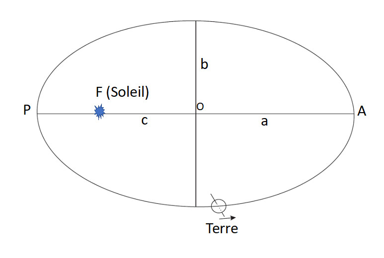
As the semi-major axis is invariant, the variation of the eccentricity is accompanied by the variation of only the semi-minor axis. The latter increases with the decrease of e and ends up being equal to the semi-major axis when the eccentricity cancels. The new semi-minor axis will then decrease with the increase of e until the eccentricity reaches its maximum.
1.2. The obliquity
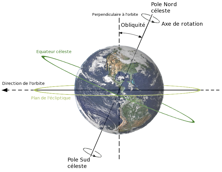
1.3. Climatic precession
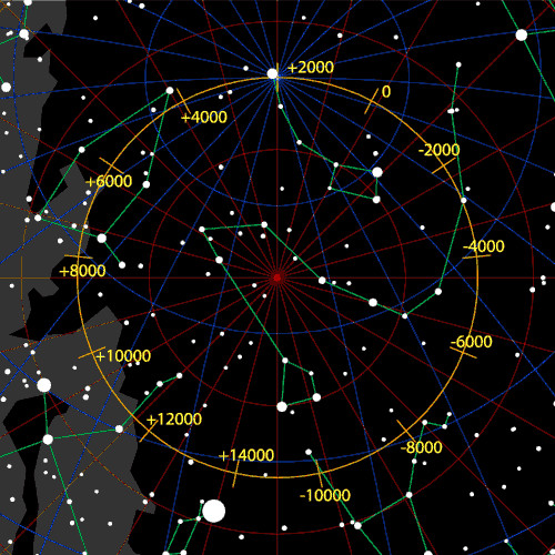
The Earth’s axis of rotation currently points to the NorthStar, Alpha Ursae Minoris in the Northern Hemisphere. This axis, in addition to the variation of its inclination on the perpendicular to the ecliptic plane, moves by forming in space an almost perfect cone whose opening is the obliquity. This movement is that of the astronomical precession, a progressive shift in the direction in which the stars are seen (Figures 4, 5 and 6) whose period is 25,760 years. It is associated with the retrograde (clockwise) movement of the vernal point on the ecliptic, which is 50.29 arc seconds per year. The latter is in fact defined at the intersection of the equator and the ecliptic (Figure 4).
![]() This average period is in fact the result of the fundamental components which are close to 23,000 years and 19,000 years and which were highlighted in the 1970 [2], thus corroborating the periods found by Hays et al [3] in the geological data.
This average period is in fact the result of the fundamental components which are close to 23,000 years and 19,000 years and which were highlighted in the 1970 [2], thus corroborating the periods found by Hays et al [3] in the geological data.
The name climatic precession was introduced [2] because it is the relative position of the vernal point in relation to the perihelion that matters in climatology and not their absolute position in the sky.
The theory that links the long-period variations of these parameters to solar irradiance on the one hand and to climates on the other hand is called the astronomical theory of paleoclimates [10],[11]. There are several versions of this theory [12] that we will describe in the context of the history of the discovery of climate variations over the last few centuries.
2. Discovering the great variations in climate
2.1. Evolution of ideas about the evolution of climates since the 18th century
Descriptive discipline, climatology has become a multidisciplinary science involving the five components of the climate system and their interactions with each other:
- the atmosphere,
- the hydrosphere,
- the cryosphere,
- the lithosphere,
- the biosphere.
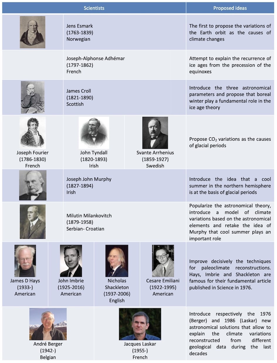
Not surprisingly, therefore, the resulting climate varies on scales ranging from seasonal to millions of years. Although this science has literally exploded in recent decades, the discovery and study of the first evidence of climate variation beyond the annual and decadal scales dates back to the 18th century. A synthesis is given in the table below.
Table. Some scientists involved in the evolution of ideas about climate change since the 18th century [13].
2.2. A first step: glacier extension and climate change
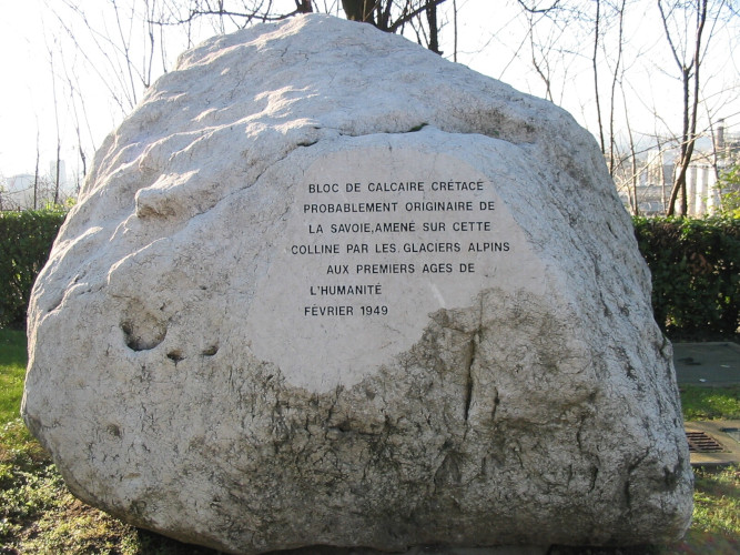
However, the location and nature of these blocks and other moraines led some scientists to admit that transport through ice would better explain the various observations. The Scottish naturalist James Hutton (1726-1797) was the first to support this idea. Others followed and discovered the imprint of climate change in the fluctuating extent of glaciers: the Swiss engineer Ignace Venetz (1788-1859), the German forest engineer Albrecht Reinhart Benhardi (1797-1849), the Swiss geologist Jean de Charpentier (1786-1855) and the German botanist Karl Fredrich Schimper (1803-1867), who introduced the notion of an ice age. However, it was the Danish-Norwegian geologist Jens Esmark (1763-1839) who, in 1824, continuing his analysis of glacier transport, proposed, most probably for the first time, that climate change was the cause of the ice age and that it was due above all to variations in the Earth’s orbit.
It was the work of these precursors that led the Swiss geologist Louis Agassiz (1801-1873) to formulate his address to the Swiss Natural Science Society in Neufchâtel in 1837 on Upon glaciers, moraines and erratic blocks. This address was criticized, however, because it appeared that Agassiz had “borrowed” his conception of glacial theory from his former university colleague Schimper and had failed to recognize Charpentier’s original contribution that introduced him to glacier research.
2.3 The Birth of the Astronomical Theory of Paleoclimates
It was also at the beginning of the 19th century that the Frenchman Joseph Adhémar (1797-1862), not content to study the polar ice caps, tried to explain in his book “Révolutions de la mer, déluges périodiques” [15] the recurrence of the ice ages from the precession of the equinoxes. The astronomical theory of paleoclimates was born and could be continued thanks to the development of celestial mechanics with the Frenchmen Jean le Rond d’Alembert (1717-1783), Jean-Baptiste Joseph Delambre (1749-1822), Pierre Simon de Laplace (1749-1827), Louis Benjamin Francoeur (1773-1849) and Urbain Le Verrier (1811-1877). At the same time, a further step was to be taken with the first calculations of the long-term variations in the energy received from the Sun, variations due to the eccentricity of the Earth’s orbit, the precession of the equinoxes and the obliquity of the ecliptic. Thus illustrating the following scientists: John Frederick William Herschel (1792-1871), L.W. Meech (1821-1912) and Chr. Wiener (1826-1896), to whom we can associate the mathematicians André-Marie Legendre (1751-1833) and Simon-Denis Poisson (1781-1840).
Everything was now ready for the Scotsman James Croll (1821-1890) to develop a theory of the ice ages based on the combined effect of the three astronomical parameters, a theory according to which the winter of the northern hemisphere was to play a decisive role. This theory was greatly appreciated by the naturalist Charles Robert Darwin (1809-1882) and taken up by the Scottish geological brothers Archibald (1835-1924) and James (1839-1914) Geikie who introduced the notion of interglacials. It is also the basis for the classification of alpine glaciations by Albrecht Penck (1858-1945) and Edouard Brückner (1862-1927) and of the American ones by Thomas Chowder Chamberlin (1843-1928). However, geologists were becoming increasingly dissatisfied with Croll’s theory and many criticisms were made.
Many refuted the astronomical theory and preferred explanations related to the planet Earth alone. The Scottish geologist Charles Lyell (1797-1875) emphasized the geographical distribution of land and sea to explain the alternation of hot and cold climates, while others turned to variations in the concentration of certain gases in the atmosphere [16]. Thus, the French physicist Joseph Fourier (1786-1830) put forward the original idea of the greenhouse effect theory related to the concentration of carbon dioxide in the air. He was followed by the Irish chemist John Tyndall (1820-1893), who was responsible for the first experiments on the absorption of infrared radiation and the hypothesis of the fundamental role played by water vapour in the greenhouse effect. Later, the Italian Luigi de Marchi (1857-1937) and the Swedish chemist Svante Arrhenius (1859-1927) proposed, along with other scientists of their time, that ice ages were due to decreases in atmospheric carbon dioxide. In 1895, Arrhenius suggested in an article published at the Stockholm Physical Society that a 40% reduction or increase in the concentration of CO2 in the atmosphere could generate feedback processes that would explain glacial advances and retreats (See From the discovery of the greenhouse effect to the IPCC).
Milankovitch was a contemporary of the geophysicist and meteorologist Alfred Wegener (1880-1930), whom he met through the Russian-German climatologist Vladimir Köppen (1846-1940). The latter had heard of Milankovitch’s work and his daughter, Elsa Köppen, had married Wegener. The modern era of the astronomical theory was born, although the lack of reliable paleoclimatic data and a reliable time scale were at the basis of many criticisms from the world of both geologists and meteorologists.
It was not until the 1950s and 1960s that new techniques made it possible to date, measure and interpret climate records in marine sediments, ice and on the continents.
In 1955, the American Cesare Emiliani [18] proposed a stratigraphy, still in force, based on the succession of minima and maxima of the oxygen-18/oxygen-16 isotope ratio measured in the shells of foraminifera found in the sediments of the deep ocean. The interpretation of this isotopic ratio was to follow in terms of salinity with Jean-Claude Duplessy [19] and in terms of temperature and ice volume with Nicholas Shackleton and Niels Opdyke [20].
Mathematical tools then made it possible to create transfer functions to quantitatively interpret the information collected in the oceans or from tree rings. The effort of the CLIMAP group [21] (1976) resulted in the first seasonal climate map of the Last Glacial Maximum and the seminal 1976 paper by James Hays, John Imbrie (1925-2016) and Nicholas Shackleton (1937-2006). The advent of large computers made possible the first climate simulations based on general circulation models [22] and the continuation of astronomical calculations led to a highly accurate reference time scale and the determination of daily and seasonal irradiation, which was essential for climate modeling [23].
3. Milankovitch’s astronomical theory and afterwards
3.1. Milankovitch and the cycles of glaciation
Its insolation curve for the boreal summer at 65°N, based on Murphy’s idea and calculated from the work of Le Verrier and Miskovitch, has remained famous (Figure 10), as it allowed geologists, Brückner, Köppen and Wegener (1925) in particular, to interpret the glacial-interglacial cycles as they knew them at that time.
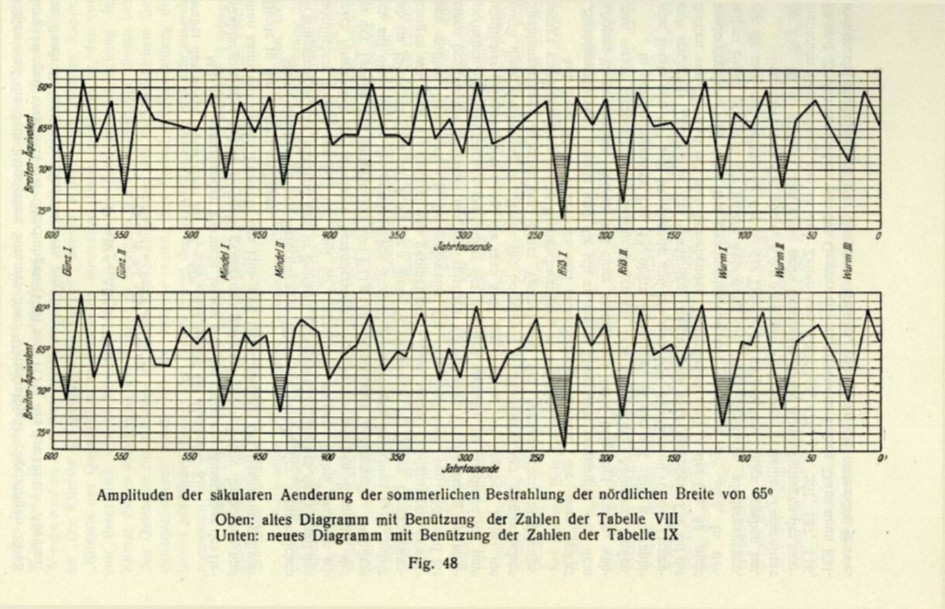
Milankovitch does not seem to have been interested in the periods which characterize the long-term variations of these astronomical parameters and simply notes, as Emiliani (1922-1995) will do in 1955 [12], [19], that the average distances between the successive maxima of his curves are for the eccentricity 92,000 years, for the obliquity 40,000 years and for the precession 21,000 years. He was also not interested in their analytical developments. In fact, it was only at the end of Milankovich’s life that the first solutions appeared allowing a more precise calculation of the astronomical elements.
3.2. More precise calculation of astronomical elements

It was then that André Berger published the trigonometric series which directly provides the spectrum of long-term variations in eccentricity, obliquity and precession, and allows a simple but precise calculation of the numerical values of these parameters over the last millions of years [25], [2]. The geological data becoming more and more reliable over the last millions and tens of millions of years have made it possible to calibrate the solutions of Jacques Laskar [26] who was the first to calculate the values of the three astronomical parameters over very long periods of time and with such precision [27]. Studies of the sensitivity of the astronomical periods to variations in the Earth’s rotation speed, the Earth-Moon distance and the dynamic ellipticity of the Earth finally showed a progressive decrease of these periods over several hundreds of millions of years [28].
The quality of the calculation of the parameters of the Earth’s orbit and its rotation achieved over the last few decades makes it possible to reproduce long-term variations in eccentricity, obliquity and climatic precession with excellent accuracy. These parameters [29] can then be used to calculate the solar energy arriving on Earth, for example during the astronomical season of a half-year of the Northern Hemisphere summer at 65°N [30]. Variations are given in Figure 11 for the last 600,000 years so that they can be compared with similar variations described by Milankovitch (Figure 10). This comparison makes it possible to assess the quality of the Milankovitch curve obtained a hundred years ago and representing the same energy available in summer at 65°N. But it also highlights the improvement of the time scale and shows a finer structure of the variations.
As mentioned above, it was the Irishman Joseph John Murphy who first proposed in 1869 that a long, cool summer and a short, mild winter would be the most favourable conditions for entering the ice age. Milankovitch popularized and propagated the idea by considering insolation at 65°N. This idea of considering high boreal latitudes stems from his work on the influence of snowfields, ice and ice caps on climate. It is in these polar latitudes of the northern hemisphere that one finds vast continental expanses allowing the installation of immense ice sheets with significant positive feedbacks allowing a significant intensification of the insolation forcing. Figure 11 suggests that periodic variations in astronomical parameters are at the origin of cyclical climate variations in the past (astronomical theory of climate). In particular, the cyclicity of the 100,000-year ice ages of the last hundreds of thousands of years [4] is correlated with eccentricity.
4. Messages to remember
- The astronomical theory of paleoclimates and its various versions have unquestionably helped to understand the climatic variations of the last millions of years and, in particular, the recurrence of glacial-interglacial cycles of the Quaternary [31].
- The parameters of the Earth’s motion around the Sun (eccentricity of its elliptical trajectory, obliquity and precession of its axis of rotation) are responsible for the natural climatic variations in the last millions of years.
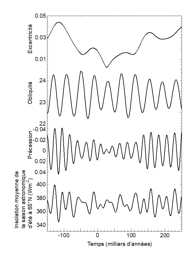
- This adventure began more than three centuries ago. It has made it possible to progressively clarify the framework within which the current climate varies and thus to better define the possible impact of human activities on the climate of the coming millennia [32]. Figure 12 reproduces the variations in astronomical parameters between 150,000 years in the past and 250,000 years in the future. Note that over the next 50,000 years, obliquity, but especially eccentricity, will decrease, with the Earth’s orbit becoming circular in about 27,000 years. This has a direct impact on climate precession, which varies very little over the next tens of thousands of years. This stability is visibly reflected in the evolution of insolation with a possible impact on the climate, as other forcings, such as greenhouse gases, could then exert a greater influence on the climate.
Notes and References
Cover image : Sequence of loess-paleosol near Xian, Shaanxi Province, China. The red layer in the middle of the picture corresponds to the interglacial MIS-9, 330 000 years ago (source: authors)
[1] Joussaume S., 1993. Climate from yesterday to tomorrow. CNRS éditions/CEA, Paris
[2] Berger A., 1978. Long-term variations of daily insolation and Quaternary climatic changes. J. Atmos. Sci, 35(12),2362-2367.
[4] Hays J.D., Imbrie J. & Shackleton N.J., 1976. Variations in the earth’s orbit: pacemaker of the ice ages. Science 194: 1121-1132. http://www.jstor.org/stable/1743620?origin=JSTOR-pdf
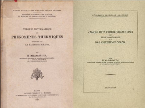
[5] Milankovitch M., 1941. Kanon der Erdbastrahlung und seine Anwendung auf des Eiszeitenproblem. Special Publication 132, Section of Mathematical and Natural Sciences, Vol. 33, p. 633. Belgrad, Royal Serbian Academy of Sciences. (‘Canon of Insolation and the Ice-Age Problem’, translated from German by the Israel Program for Scientific Translations and published for the U.S. Department of Commerce and the National Science Foundation, Washington DC, 1969. Reprinted by Zavod za udzbenike i nastavna sredstva in cooperation with Muzej nauke i tehnike Srpske akademije nauka i umetnosti, Beograd, 1998).
[6] Johannes Kepler (1571-1630), astronomer. https://www.astrofiles.net/astronomie-johannes-kepler
[7] Perihelion and aphelion are the places in the Earth’s orbit around the Sun where the Earth-Sun distance is the shortest and the longest respectively. If rp is the distance to perihelion and ra to aphelion, the ellipse equation gives rp = a(1-e), ra = a(1+e) et ra– rp = 2ae.
[8] Irradiance is expressed in Watts per m2, it is the quantity of energy, in Joules, which passes per unit of time, the second, perpendicularly through a unit of surface, one m2 and this, at the average distance Earth-Sun.
[9] The word insolation is an abbreviation for incoming solar radiation.
[10] Imbrie, J., Imbrie, K. P., 1979. Ice Ages, Solving the Mystery. Enslow Publishers, New Jersey.
Berger, A. 1988. Milankovitch theory and climate. Reviews of Geophysics 26(4): 624-657.
Berger,A., 2012. A brief history of the astronomical theories of paleoclimates. In: “Climate change at the eve of the second decade of the century. Inferences from paleoclimates and regional aspects”. Proceedings of Milankovitch 130th Anniversary Symposium, A. Berger, F. Mesinger, D. Sijacki (eds). 107-129. Springer-Verlag/Wien.DOI 10.1007/978-3-7091-0973-1.
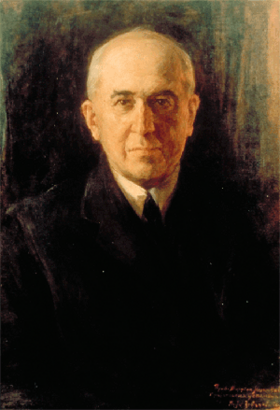
[13] The sources of the engravings or photos in the table are as follows: Jens Esmark (engraving Louis Fehr / Public domain, via Wikipedia Commons); James Croll (photo Luis Alberto 9919 / CC BY 3.0, via Wikipedia Commons); Joseph Fourier (engraving Amédée Félix Barthélemy Geille / Public domain, via Wikipedia Commons); John Tyndall (Woodburytype by Lock and Whitfield, no copyright, United States, CC0, via The Sminthonian Libraries); Svante Arrhenius (Photogravure Meisenbach Riffarth & Co. Leipzig. / Public domain, via Wikimedia Commons); Joseph John Murphy (Photo reproduced from Complex adaptations, University of Utah); Milutin Milankovitch (Portrait at the Serbian Academy of Sciences and Arts in Belgrade, painted by Paja Jovanovic in 1943 [source frwiki / CC BY-SA 3.0]); James D Hays (Columbia University); John Imbrie (Columbia University); Nicholas Shackleton (source frwiki / CC-BY-SA); Cesare Emiliani (Universal Holocene Calendar, Facebook); André Berger (photo André Berger); Jacques Laskar (photo https://perso.imcce.fr/jacques-laskar/en/)
[14] References to ancient texts are given in Berger (reference [12]).
[15] Adhémar, J. A., 1842. Revolution of the Seas, Periodic Floods. First edition: Carilian-Goeury et V. Dalmont, Paris. Second edition: Lacroix-Comon, Hachette et Cie, Dalmont et Dunod, Paris, 359 p.
[16] Bard, E., 2004. Greenhouse effect and ice ages: historical perspective. C. R. Geoscience, 336, 603-638.
[17] Milankovitch, M., 1920. Mathematical Theory of Thermal Phenomena Produced by Solar Radiation. Yugoslav Academy of Sciences and Arts in Zagreb (Gauthier Villars, Paris).
[18] Emiliani, C. R. W., 1955. Pleistocene temperatures. Journal of Geology 63(6): 538-578.
[19] Duplessy, J. C., 1970. Preliminary note on variations in the isotopic composition of the Indian Ocean in the O18-salinity relationship. C. R. Académie des Sciences de Paris, 271 series D, 1075-1078.
[20] Shackleton, N. J. and Opdyke, N. D., 1973. Oxygen isotope and paleomagnetic stratigraphy of equatorial Pacific core V28-238: Oxygen isotope temperatures and ice volumes on a 105 and 106 year scale. Quaternary Research 3: 39-55.
[21] CLIMAP Project Members. 1976. The surface of the Ice-Age Earth. Science 191: 1131-1136.
[22] Alyea, F.N., 1972. Numerical simulation of an ice-age paleoclimate. Atmosphere Science Papers 193, Colorado State University, Fort Collins, USA.
[23] Berger A., 1973. Astronomical theory of paleoclimates. Doctoral dissertation, Catholic University of Louvain, Faculty of Sciences, 2 volumes.
[24] Bretagnon, P., 1974. Long-term terms in the solar system. Astronomy and Astrophysics 30: 141-154.
Berger, A., 1976. Obliquity and general precession for the last 5 000 000 years. Astronomy and Astrophysics, 51, pp. 127-135.
[26] Laskar J., 1986, Secular terms of classical planetary theories using the results of general theory, Astronomy and Astrophysics, 157, 59-70.
[27] Laskar J., Fienga A., Gastineau M. & Manche H., 2011. La2010: a new orbital solution for the long-term motion of the Earth. Astronomy and Astrophysics, 532, A89, 1-15. 0. EDP Sciences, 1051/0004-6361/201116836
[28] Berger A., Loutre M.F. & Laskar J., 1992. Stability of the astronomical frequencies over the Earth’s history for paleoclimate studies. Science, 255, pp. 560-566.
[29] Berger A. and Loutre M.F., 1991. Insolation values for the climate of the last 10 million years. Quaternary Science Reviews, 10 n°4, pp. 297-317.
[30] Berger A., Loutre M.F. and YIN Q.Z., 2010. Total irradiation during the interval of the year using elliptical integrals. Quaternary Science Reviews, 29, pp. 1968-1982. doi:10.1016/j.quascirev.2010.05.007
[31] Yin Q.Z. & A. Berger, 2012. Individual contribution of insolation andCO2 to the diversity of the interglacial climates of the past 800,000 years, Climate Dynamics, 38, 709-724. DOI 10.1007/s00382-011-1013-5
[32] Berger A. & M.F. Loutre, 2002. An Exceptionally long Interglacial Ahead? Science, 297, pp. 1287-1288
The Encyclopedia of the Environment by the Association des Encyclopédies de l'Environnement et de l'Énergie (www.a3e.fr), contractually linked to the University of Grenoble Alpes and Grenoble INP, and sponsored by the French Academy of Sciences.
To cite this article: BERGER André, YIN Qiuzhen (January 5, 2025), Astronomical theories of climate: a long history, Encyclopedia of the Environment, Accessed July 23, 2026 [online ISSN 2555-0950] url : https://www.encyclopedie-environnement.org/en/climate/astronomical-theories-of-climate-long-history/.
The articles in the Encyclopedia of the Environment are made available under the terms of the Creative Commons BY-NC-SA license, which authorizes reproduction subject to: citing the source, not making commercial use of them, sharing identical initial conditions, reproducing at each reuse or distribution the mention of this Creative Commons BY-NC-SA license.