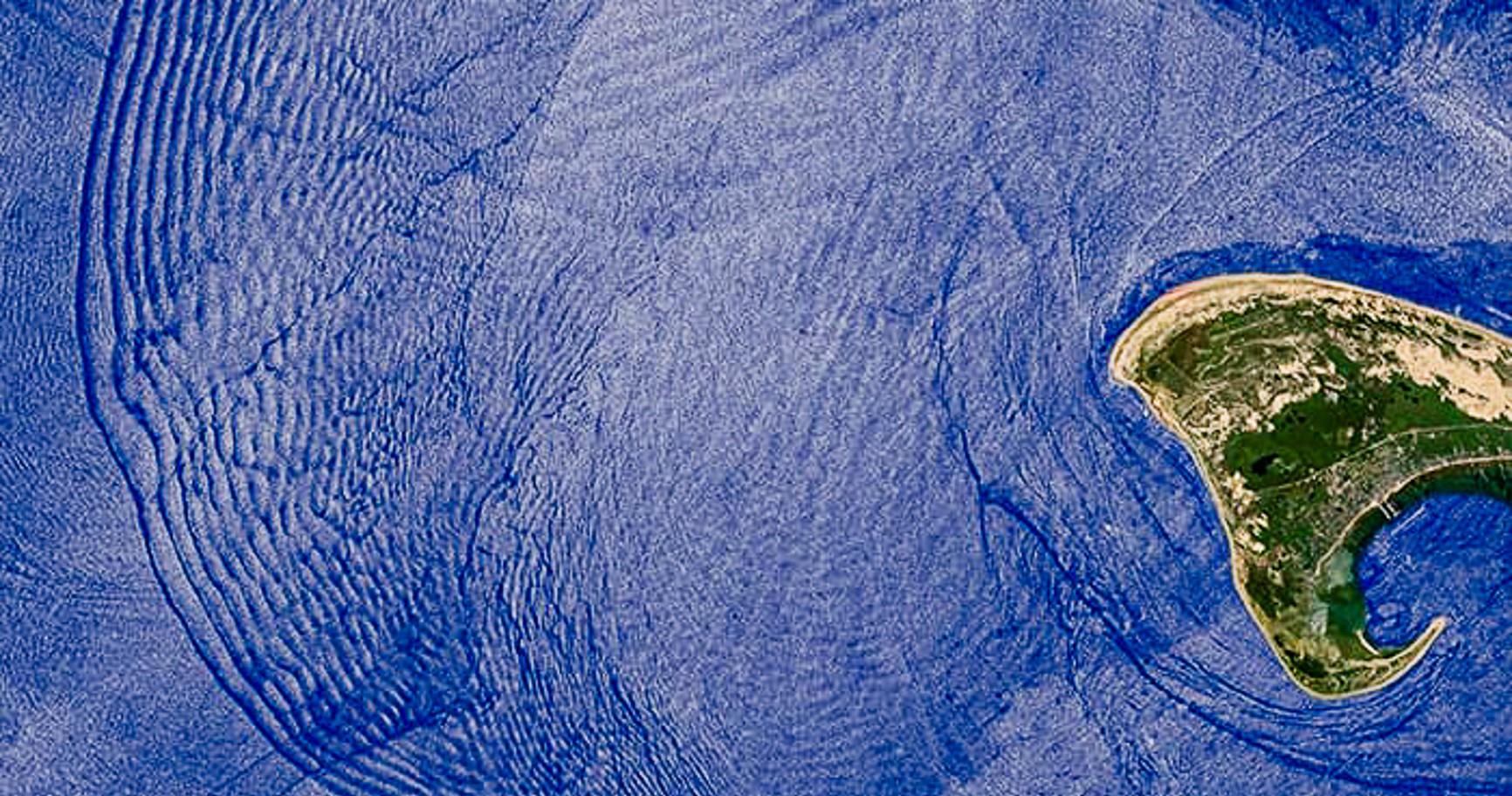
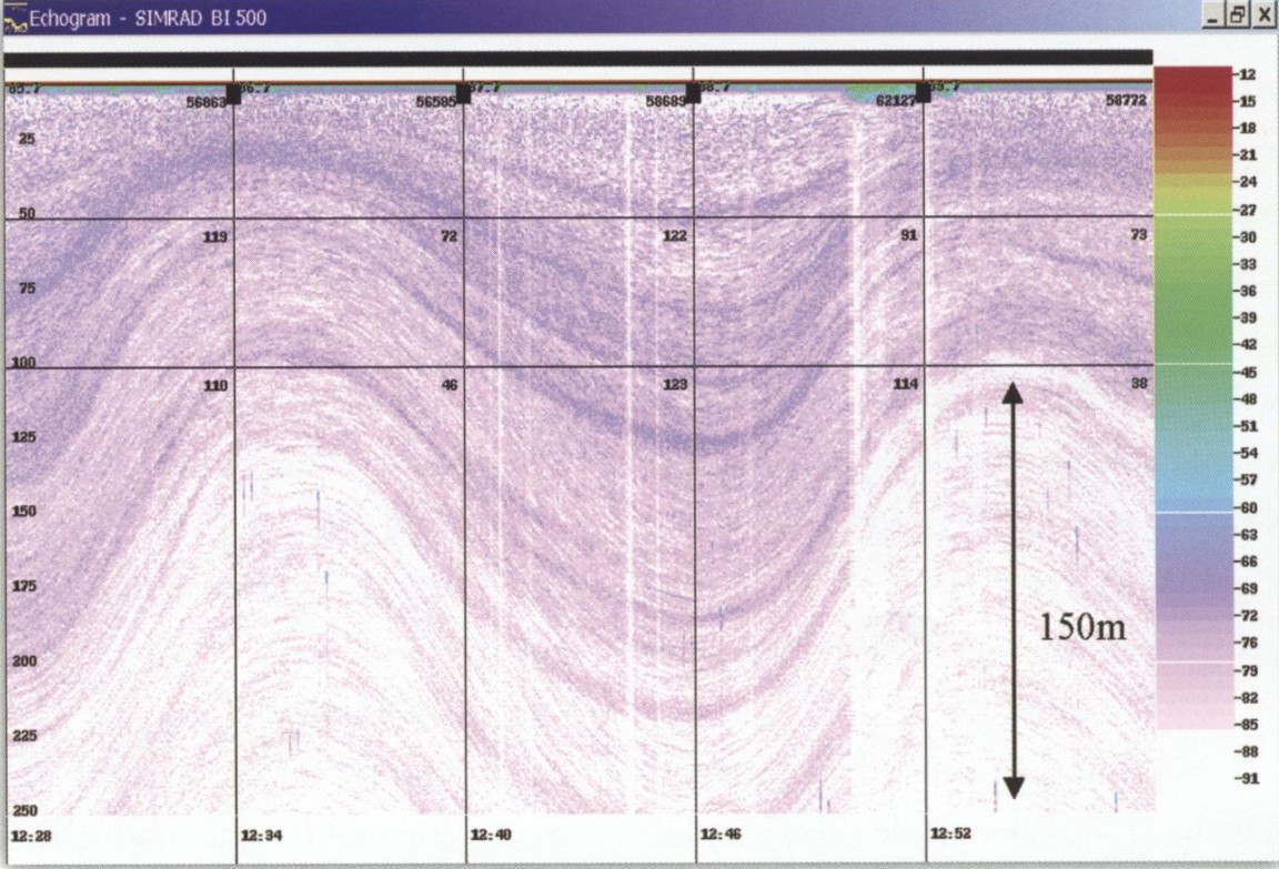
Waves are not limited to the sea surface. They propagate in the deep ocean as disturbances of the density layers set by the vertical profiles of temperature and salinity. These so-called internal gravity waves exhibit larger amplitudes (up to 300 m) and lower frequencies compared to ocean surface waves because of their reduced restoring force. They are commonly generated by wind gusts and by the uplift of oceanic currents over sea bed topography. Thus, isolated sea mounts, mid-ocean ridges and continental slopes can be sources of internal waves under proper conditions. Internal waves occur in the form of periodic internal tides, but are also scattered as a random superposition of small-scale waves. Internal wave activities pose safety hazards to marine structures, contribute to background noise in underwater sound channels, and act as a mixer of deep-sea water. Internal waves are therefore involved in many fields of marine science and engineering.

 

1. Giant underwater wave

Because of dilatation, warm water is lighter than cold water, so it floats and remains near the surface. Moreover, salty water is denser than fresh water, so that density depends both on temperature and salinity. In a stable configuration, water layers are sorted in density, which continuously increases with depth. Vertical density gradients are often concentrated in a zone called pycnoclinepycnocline, in oceanography, boundary separating two liquid layers of different densities. In oceans a large density difference between surface waters (or upper 100 metres [330 feet]) and deep ocean water effectively prevents vertical currents; the one exception is in polar regions where pycnocline is absent., separating two layers with quasi-uniform density, a lighter top layer and a denser bottom layer. Waves can propagate along this interface in a very similar way as surface waves. In the more general continuously stratified case, waves can also propagate along a direction tilted with respect to the horizontal.

Since internal waves occur inside the water body, their existence is not easily perceived, which makes their observation and study shrouded in a layer of mystery. During an Arctic expedition in 1893, the famous Norwegian scientist and polar explorer Fridtjof Nansen observed that his research ship Fram suddenly slowed down in the North of Siberia.  This occurred near the coast of Taymyr Peninsula while the ship was navigating through an area of fresh water formed by melting ice, floating on the underlying sea water. His report [1] was the first scientific description of a phenomenon called ‘dead water’. This was however mentioned earlier in sailor tales.

The phenomenon has been explained in 1904 by the Swedish oceanographer and physicist Vagn Walfrid Ekman in his PhD thesis [2]: it is due to the formation of waves at the density interface between salty and fresh water. In suitable conditions, the wake produced at this interface can be of much higher amplitude than the usual surface wake, resulting in considerable energy expense and difficulty to move forward. This was the early discovery of internal waves in the ocean.

VIDEO  Link to the movie https://culturesciencesphysique.ens-lyon.fr/images/articles/eauxmortes/phenomene-eaux-mortes-deux-couches.webm)

Ekman was able to reproduce the phenomenon in the laboratory, in an experiment reproduced with modern tools in Figure 1. In 1847, the British physicist George Gabriel Stokes had previously proposed the theory of interfacial waves between two layers [3], a direct generalisation of his seminal work on surface waves. In 1883, Lord Rayleigh studied the case of continuous stratification, where waves can propagate in a direction slanted with respect to the horizontal.

Internal waves are commonly observed also in the atmosphere as vertically oscillating wind downstream a mountain. This can be nicely visualised by lenticular clouds, as shown in Figure 1. These waves often overturn and break, producing spots of turbulence like water waves on the beach. This is a source of clear air turbulence encountered in aircrafts.

In the case of underwater waves, little progress was made over a long period of time due to the difficulty of observation. In the 1960s, advances in detection facilitated theoretical and applied research on internal waves. Exxon Company discovered in the 1970s, after four months of observations and following drilling operations in the Andaman Sea (Indian Ocean) that the sea could have flow speeds as high as 1.8 m/s. Subsequent satellite images showed that internal waves had passed through the area [4]. These images, shown in Figure 2, are obtained by a technique called Synthetic Aperture Radar (SAR). This technique probes the capability of the sea surface to diffuse the reflected radio waves, which itself depends on the sea roughness. The sea currents associated with internal waves perturb the propagation of surface waves whose texture therefore provide a footprint of the internal waves.

Amoco Company also noticed internal tides in the South China Sea – i.e., internal waves induced by tidal currents passing through the seafloor topography. Therefore, the power of these hidden underwater waves must not be taken lightly.

Why is it that the same external factors causing only small disturbances on the surface of the ocean, can set off huge waves in the ocean?  The density difference (or gravity and buoyancy difference) in the stratified ocean is much smaller than that between the atmosphere and seawater. Consequently, the restoring force, which is proportional to the density difference, is significantly reduced to about 0.1% of that for surface waves. This reduction results in an increase in wave amplitude. Therefore, the amplitude of the internal waves can reach up to over 100 meters, 20 to 30 times that of the surface waves. Internal wave periods of oscillation range from a few minutes to dozens of hours.  Wavelengths typically range from hundreds of meters to tens of kilometers. Therefore, internal waves are huge underwater waves. For the same reason, internal waves propagate slowly, with a phase speed of the order of 1 m/s, while the induced current speed can reach 2 m/s.

2. Density Stratification of the ocean

Understanding the density stratified structure of the ocean is the prerequisite for exploring the mechanism of the formation of internal waves. Salinity effects are limited to specific locations, and water density is more generally controlled by temperature. The ocean can be broadly divided into three vertical layers. The Upper Mixed Layer (UML), typically a few dozen meters thick, is strongly mixed by wind shear and surface wave breaking. Turbulent mixing within this layer results in a nearly uniform temperature distribution. At the seafloor, the Bottom Boundary Layer (BBL), about 10 meters thick, is similarly mixed by the turbulence due to flow shear. Between these two layers lies the mesosphere, a relatively calm region within the ocean interior. In this region, density layers undergo gentle oscillations by internal waves, but turbulence is sporadically produced by wave breaking process [5], somewhat similar to surface wave breaking.

Between the upper mixed layer and the deep water there exists a thermocline with a large temperature difference (hence a large density step) that virtually prevents the transfer of momentum, energy and mass between the upper and lower water bodies. There are two types of thermoclines as follows:

• The permanent thermocline: its depth（about 100-800 meters）and intensity do not vary with season, but depends on latitude. Near the equator, the thermocline is shallower and intense; it becomes deeper and less intense at higher latitudes, and can even disappear in the Arctic region.
• The seasonal thermocline: it occurs in summer and autumn by direct solar heating, with depths of around 100 meters, as shown in Figure 3 (See The marine environment).

The thermocline tends to spread downward by mixing process stemming from the Upper Mixed Layer by wind stress, heating and cooling. This downward spreading is balanced in average by slow uplift due to ocean circulation. The deep ocean is indeed permanently filled with cold water coming from polar regions, as it will be discussed in section 7.

With the improvement of the accuracy of detection, additional lamellar microstructures of density have also been discovered in thermocline and deep water.  Their thickness is 2~10 m and horizontal extension 2~20 km. The formation mechanism of this jagged microstructural layers has yet to be further explored. It could be attributed to the interaction between different water masses and the breaking of small-scale internal waves.

3. Detection and spatiotemporal distribution of internal waves

Satellite observation using Synthetic Aperture Radar (SAR) provide global visualisation of the wave patterns by the associated sea roughness, as already shown in Figure 2. Note that sea roughness can be also directly seen by the diffusion of solar light, but SAR is highly sensitive and unaffected by clouds and sunlight, making it the primary means of detection. However, it does not provide a quantitative measurement of the wave structure.

Time records from buoy arrays, fixed ocean platforms and research vessels provide more precise information at particular locations. Vertical density profiles are provided by chains of temperature/salinity sensors, while the associated velocity profile is measured by its influence on ultrasound propagation, using Acoustic Doppler Current Profilers (ADCP).

Since 1960, traces of internal waves have been successively detected in ocean waters using those various sensors, thus promoting the study of internal waves. Remote sensing and on-site observation by various countries on the ERST/LAND STAT-1 space station have made it possible to map the global distribution of internal waves. It has been found that most of the internal waves occur in marginal regions of the oceans where the stratification, topography and ocean currents are suitable. These currents are mainly produced by tides (See The tides), and the resulting internal tides propagate at a speed of typically 1 m/s. With a 12 hours period, their wavelength is typically 50 km. However, they tend to concentrate into trains of solitary waves whose length is reduced to the km scale, as discussed in next section (Figure 4).

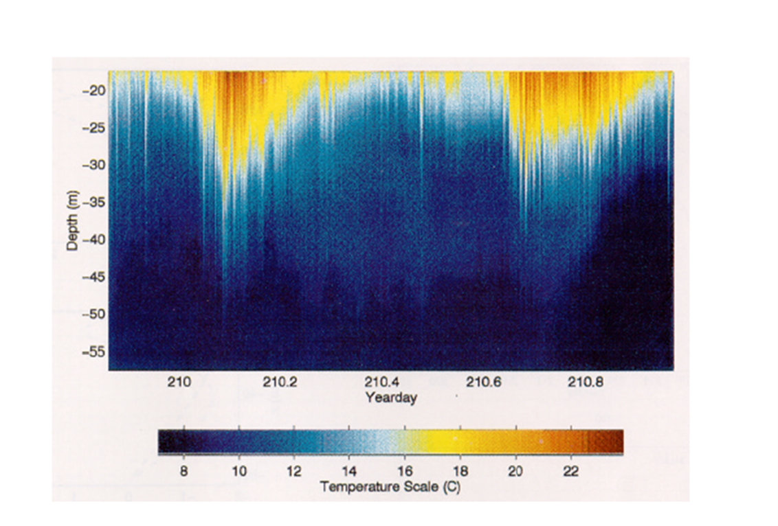
One of the most active areas of internal tides is located in the northern part of the South China Sea, in the Luzon Strait. Several factors contribute this prevalence. Those include the seasonal thermocline that develops in spring and summer, the gradually shallowing topography from southeast to northwest, and the narrow waterways in the eastern Philippines. The interaction between barotropic tides and the complex topography generates large waves or splits [6].

The ocean waters where internal waves occur can extend to as far as Bering Strait in the Arctic and the Weddel Sea in the Antarctic. Beside marginal seas, internal waves can be generated from isolated sea mounts or ridges. They are noticeably observed north of the Azores on and mid-Atlantic ridge, and northeast of the Bismark-Solomon Islands in the South Pacific. The former is caused by the passage of the current of Mexico Gulf over the seafloor ridge, while the latter is attributed to the presence of sills between the Bismark-Solomon Islands [7].

Note that in addition to these organized topographic sources, internal waves are produced in a random way by wind fluctuations which drive surface currents. This results in a continuous spectrum of internal waves filling the whole ocean, but particularly active after storms. Wind forcing is also important in lakes. The proper period of the internal sloshing motion is often close to one day, so it is prone to resonant excitation by the daily period of thermal wind.

4. Various forms of internal wave

Internal waves can take a wide variety of forms, like surface waves. They can propagate as gentle sine shape undulations at small amplitude, or take specific shapes associated with nonlinear effects at large amplitude (See Waves and swells).  A remarkable process is the formation of trains of solitary waves by the steepening of the internal tides, initially produced as tidal currents pass over topography [8]. This is shown in Figure 5.

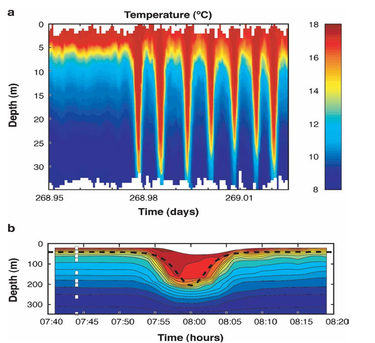
In 1834, the Scottish scientist John Scott Russell observed an astonishing wave rising from the water surface in front of a ship in a canal. It takes the form of an isolated elevation which propagates on long distance without change of shape. This is remarkable since such an isolated bump is usually described as a superposition of different wavelengths, each of which propagating at different speed. This should result in a splitting of the bump into wave trains.  This dispersive effect is in fact balanced by a steepening due to nonlinear effects, which sets the steady shape of this so-called solitary wave.

This initial observation by Russell has been long ignored, and its importance recognised only in the middle of the 20^th century. It is now recognized as a fundamental process with deep implications in mathematics and physics. The splitting of tidal waves into a train of solitons is now well understood by theory [9].

5. Safety hazards of marine structures

In order to meet energy needs, the first offshore platform was launched in the Mexico Bay in 1947. In the following decades, more than 1,000 offshore platforms were erected in the Gulf of Mexico, Northern Europe, West Africa, South America, the South China Sea and other regions. As water depths range from tens to 3,000 meters, the platforms vary from jacket, compliant to floating ones, see Figure 6.  In the severe oceanic environment of wind, wave and current, the external loads to which the platforms are subjected must be considered for the safety of platforms and personnel in operation.  The internal wave loads are one of the most significant factors [10].

Through the analysis of internal wave flow field, the following conclusions can be drawn: velocity shear occurs above and below the pycnocline. The density difference between the upper and lower layers of the pycnocline influences its properties: a larger density difference leads to a thinner pycnocline and stronger shear. This conclusion has been validated by observations in the Messina Channel, located in Sicily, in the Mediterranean Sea.

Internal waves are also safety hazards for underwater vehicles. There are records of underwater vehicles falling to the bottom, and enquiry concluded that the reason was that the vehicle encountered a strong internal wave. The dramatic vertical force dragged it to the bottom of the ocean, where it was unable to withstand the extreme pressure and then broke into pieces. Therefore, the crew of underwater vehicles must always be alert to avoid internal waves, so as to adjust the hull balance in time and avoid accidents.

6. Source of background noise in the underwater sound channel

The absorption attenuation rate of underwater sound can be less than 0.1 dB/km (at 1kHz), which means that the power decreases by a factor 10 over 100 km. This is at least 1000 times less than electromagnetic waves, so that sound waves are the most favored means of underwater detection. After the shipwreck of the Titanic in 1912, USA scientists invented an instrument for detecting underwater targets via sound echoes. In 1914, an underwater iceberg was detected 3000 m away.  With the invention of piezoelectric transducers, combined with electron tube amplification technology, the use of underwater sound for long-distance detection became operational. During the first world war, the French physicist Paul Langevin developed the sonar, pioneering modern underwater acoustics . The technology has been widely applied in the detection of ships, fish, water depth, landform, and oil reservoirs (Figure 7) [11], [12].

Beside absorption, the wave intensity decreases by geometrical spreading. However, this process is reduced by a phenomenon of wave channel similar to the guiding of light in optical fibers. Indeed, the sound speed depends on the temperature and pressure of seawater, which leads to wave deflection by refraction. In the main thermocline, extending from the water surface to a depth of several hundred meters, the sound speed decreases with depth, due to lower temperature. At still higher depth, the temperature becomes nearly uniform and the effect of pressure dominates, resulting in a sound speed increase with depth. The sound speed therefore reaches a minimum below the thermocline, which traps sound waves by refraction. The sound waves can travel a long distance along these guiding channels, and the detection distance can exceed thousands of kilometers.

Sound waves provide much information on targets. The target itself can emit sound, or it can just reflect the incoming sound. The latter corresponds to active detection, in contrast with passive detection. The reflection signal depends on the target shape, elastic properties and speed. The latter can be measured by the induced frequency shift of the reflected sound with respect to the incoming sound (Doppler shift).

In active detection, the spectral characteristics of the emitted sound provides much information. Blade vibrations caused by water flow emit sound at specific frequencies (line spectrum) while the process of cavitation emits noise over a broad band frequency range, with spectral peak in the 100-1000 Hz interval.

The acoustic signal is perturbed by background noise and reverberation effects along propagation lines. Internal waves have a strong influence in this respect. They can produce a factor 10 in signal intensity.  This can be used to explore regular and random internal wave properties.

7. Deep water mixing “agitator”

The horizontal movement of ocean currents is driven by wind stress, while gravity effects are at stake in the thermohaline circulation. The latter involves the sinking of dense water in polar regions, particularly in the Denmark Strait between Iceland and Groenland. This sinking is fed near surface by the Gulf-Stream, which has acquired excess salinity by evaporation on its way through tropical regions. This incoming water thus acquires a density excess after it is cooled at the contact of the atmosphere in Arctic Sea, which allows its sinking to the deep ocean.

The global result is a meridional loop carrying warm surface water poleward while the deep cold water somewhat finds its way upward at lower latitudes, closing the loop (See The slow and powerful ocean circulation). This thermohaline circulation provides a global heat flux from equator to pole, of similar magnitude as the atmospheric circulation. Therefore, it significantly tempers the climate over the Earth (See The climate machine). It also influences climate through the dissolution and sequestration of carbon dioxide in the deep ocean (See A carbon cycle disrupted by human activities).

The thermohaline circulation has also a key ecological role for the survival and reproduction of organisms (Figure 8). Indeed, it brings dissolved oxygen to the deep ocean while it lifts fertilising chemicals and nutriments from the sea floor to the surface.

Note that the thermohaline circulation requires some mechanical energy input. As early as 1916, the Swedish scientist Johan Wilhelm Sandström has proved that this circulation cannot be maintained just by gravity from cold and heat sources located at the same horizontal level: conversion from thermal to mechanical energy requires that heating occurs at lower altitude than cooling. This is indeed the case for atmospheric motion, which is globally driven by gravity effects. The result of Sandström has been revisited more recently with refined hypothesis, but it still remains basically valid.

The mechanical input needed to maintain the thermohaline circulation comes mainly from the vertical mixing by internal waves. This mixing indeed globally lifts cold heavy fluid from the bottom toward the surface, closing the thermohaline circulation against gravity. Note that the internal waves themselves only involve reversible oscillating motion, but mixing occurs when the waves break and release their energy in the form of turbulence.

The energy responsible for deep water mixing mainly comes from the wind and tides [13]. The wind power input to the ocean is estimated as 20 TW (20 10¹² watts), mainly as surface waves. Only a few percent drive ocean currents and large horizontal eddies. Wind fluctuations also generate internal waves with a power about 0.6 TW.

The other source of internal waves is the tide which provides globally an energy of 3.5 TW to ocean currents, from which 25% (0.9 TW) is converted to internal tide by interaction with topography. These estimates, still very unprecise, indicate that the internal waves globally receive a power of the order 1 TW, about half from the wind and half from the tides. About 25 % of this power (the mixing efficiency) is used to maintain the thermohaline circulation by vertical mixing.

8. Messages to remember

• The ocean maintains a stable density stratification structure, and internal waves are the manifestation of pycnocline disturbances. Compared with surface waves, internal waves are characterized by larger amplitude, longer period, slower propagation.
• Under the external disturbance such as wind, air pressure, tides, seabed landslides and object movements, various forms of internal waves can be induced under appropriate stratified structure and terrain conditions, including micro-amplitude waves, nonlinear internal waves, solitary waves (clusters), internal wavelet package, internal tides, etc.
• Internal waves are a hidden danger to the safety of marine structures, a source of noise for underwater acoustic detection and an “agitator” for deep-sea circulation, so the study of internal waves is of great scientific and engineering significance.
  

  ---

  Notes & references

  Cover image. Dutch Boats in a Gale by Joseph Mallord William Turner (1775–1851), 1801 [Source Joseph Mallord William Turner, Public domain, via Wikimedia Commons]

[1] Nansen F. (1897), Farthest North,  https://www.gutenberg.org/files/30197/30197-h/30197-h.htm

[2] Ekman V. W. (1904), On dead water, Norw. N. Polar Exped. 1893–1896: Sci. Results, XV, Christiana, Ph.D. thesis.

[3] G. Stokes (1847), On the Theory of Oscillatory Waves, Transactions of the Cambridge Philosophical Society VIII, 197–229, and Supplement 314–326.

[4] Osborne A.R., Burch T.L. (1980), Internal solitons in the Andaman Sea, Science, 208:

[5] Li J.C. (1993) Turbulence in Atmosphere and Ocean. In: New Trends on Fluid Mechanics and Theoretical Physics, Peking University Press,1993, 427-433

[6] Cai S.Q., Gan Z.J., Long X.M. (2001) Some Characteristics and evolvement of the internal soliton in the northern South China Sea. Chinese Science Bulletin, 46（15),1245-1250 – Orr M.H., Mignerey PC. (2003) Nonlinear internal waves in the South China Sea: observation of the conversion of depression internal waves to elevation internal waves. J Geophys. Res. 108（C3, 3064-3076.

[7] Jackson C.R., Apel J.R. (2002), An Atlas of Internal Waves and Their Properties. Global Ocean Associates.

[8] Grimshaw R. (1997), Internal solitary waves. In: Liu Philip L-F, Eds. Advances in Coastal and Ocean Engineering. Vol. 3 World Scientific. 1-30.

[9] Helfrich K.R. & Melville W.K. (2006), long nonlinear internal waves, Ann. Rev. Fluid Mech. 38, 395-425 – Duda T.F. et al. (2004), Internal tide and nonlinear wave behavior in the continental slope in the northern South China Sea. IEEE J. Ocean Eng. 29, 1105-31.

[10] Sarpkaya T, Isaacson M (1981), Mechanics of Wave Forces on Off-shore Structures. New York: Van Nostrand Reinhold – Chakrabarti S.K. (1994), Fluid Structure Interaction in Offshore Engineering. Computational Mechanics Publication.

[11]  Susanto R.D., Mitnik L., & Zheng Q. (2005). Ocean internal waves observed in the Lombok Strait. Oceanogr., 18(4):80{87.

[12] Caruthers JW. Elementals of Marine Acoustics. Elsevier Company, 1977

[13] Wunsch C, Ferrari R. (2004) Vertical mixing, energy and the general circulation of the oceans. Ann Review of Fluid Mech. 36: 281~304