The climate machine

This general introduction presents some basic concepts that will allow the reader to gain an overview of the climate machine, i.e. how the climate system works and why it is so complex. First, we will define what the word “climate” means (clearly distinguishing it from meteorology) and then we will present a synthetic vision of the essential components of the climate system. The concepts of forcing and feedback make it possible to clearly distinguish external and internal effects and mechanisms that cause climate change. The issue of climate predictability at different time scales is then discussed. Finally, there is a brief introduction to the working methods used in climatology and the many related disciplines (physics, geology, chemistry, biology,…).

1. What is climate?

Climate is often defined by average weather conditions (temperature, rain, wind, etc.), or rather as a statistical description of “time” in terms of means and variability (fluctuations, trends, frequencies and intensity of extremes), for time periods beyond the month. Typically these statistics are calculated over a period of 30 years. Meteorology, a scientific discipline close to climatology, concerns the forecasting of weather with shorter deadlines, below the month. The physical quantities taken into account are of course temperature, but also precipitation, cloud cover, wind speed and direction, etc. (read Introduction to weather forecasting).

The need to consider durations of several decades comes from the large variability of the climate system. Thus, the global average temperature can typically vary by 0.2°C from one year to the next (Figure 1, [1] ); at a given location, the amplitude of this interannual variability can exceed several degrees (Figure 2). There are typical structures (called “modes”) of spatial or temporal variability such as the Austral-El Niño Oscillation (ENSO) or the Decadal Pacific Oscillation. The term “oscillation” here indicates that these are repetitive phenomena (but in reality without a well-defined frequency); often these modes of variability are centred on a particular place on the globe, as their name suggests.

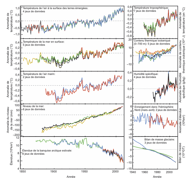
Globally, the Earth’s climate has varied, varies and will vary at all scales of time, from the hundred million years to the decade. The global average surface temperature and the global volume of ice (through its effect on sea level: the more ice is placed on the continents in the form of ice caps such as those of Greenland or Antarctica at present, the lower the global sea level) are naturally the preferred indicators for characterizing climate and its variability.

At a more local scale, all climate-influenced environmental characteristics (mountain glaciers, vegetation, lakes, etc.) can be used as climate indicators (Figure 1). Traces of the past state of these natural elements are used to “reconstruct” climates from past periods for which we do not have weather records.

2. Why “climate machine”?

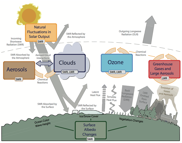
The sun is the source of energy essential for the climate system. About half of the sun’s radiation is absorbed by the Earth’s surface, the other half being either reflected back into space (about 30%) or absorbed directly into the atmosphere (the remaining 20%). The absorbed radiation heats the Earth’s surface. However, any body emits so-called “thermal” radiation, depending on its temperature: the hotter it is, the higher its thermal radiation is. At the temperatures typical of the climate system, this thermal radiation is infra-red, invisible. The Earth’s surface and atmosphere therefore emit a thermal radiation which constitutes an outgoing energy flow. In the long term, the solar energy flux absorbed by the Earth is close to the energy flux emitted by the Earth in the form of thermal radiation. A difference between incoming and outgoing energy flows leads to a variation in the energy content of the climate system – in other words, global warming or cooling.

At the heart of the climate system, the atmosphere and oceans, through their winds and currents, distribute excess solar energy from low latitudes towards the poles, which are in deficit. It is in this sense that we can speak of a “machine”: temperature differences are converted into motion, whose kinetic energy is, of course, dissipated into heat.

Atmospheric and oceanic movements are both horizontal and vertical, although the climate system is actually a very flat system: while 80% of the mass of the atmosphere is concentrated in the first 10 kilometres above the surface, the atmosphere covers the entire surface of the Earth and is therefore measured horizontally in tens of thousands of kilometres. The same applies to the ocean, which is an average depth of 3800 m. However, the significant elements of the general circulation of the ocean and atmosphere include vertical movements, caused mainly by differences in density between water or air masses. In the atmosphere, these density differences are mainly caused by differences in temperature (and water vapour content); in the ocean, temperature and salinity are the main determinants of density differences leading to upward and downward movements.

Thus, for example, Hadley’s circulation of the atmosphere at low latitudes (read The atmospheric circulation: its organization) is characterized by an upward movement of superheated air masses from the equatorial region. These air masses cool down as they rise (by decompression), causing heavy rainfall in these areas. When they reach an altitude of about ten kilometres, these air masses move away from the equator to the north and south. The Earth’s rotation induces an eastward deviation of this horizontal movement due to the conservation of the kinetic moment and the Coriolis force. Plumbing the large subtropical desert areas, these air masses descend and warm up: this warming further reduces the relative humidity of the air, hence the low cloud cover at the origin of the formation of these deserts. At the surface, a horizontal movement opposite to that of altitude is set up and these surface winds towards the equator, diverted westward by the Coriolis force, are called trade winds (read The key role of trade winds).

Beyond these large general circulation systems, of which Hadley circulation is an iconic example, many transient systems characterize atmospheric and oceanic circulation. Thus, the succession of high and low pressure systems is a well-known element of “time” at mid-latitudes. These transient systems are, in the same way as stable circulation systems, ultimately caused by the difference in sunlight between low and high latitudes, and perform transport of energy to the poles. It is interesting to note that the ocean and atmosphere carry about the same amount of energy from the equator to the poles.

3. A complex system

Other components complete this climate system: ice (sea ice and continental ice), often referred to as “cryosphere“; living beings, including vegetation, which constitute the “biosphere“; the continental surface. The components of the system interact with each other via exchanges of energy (mainly heat, but also kinetic energy), water and carbon. Obviously, these energy, water and carbon flows also occur within each component of the climate system (read Weather forecasting models).

The reference to the carbon cycle may come as a surprise here, while the reference to energy and water flows is unlikely to surprise the novice reader: indeed, we see and feel them every day, and we easily visualize the water cycle, from its evaporation over the ocean, its transport in the atmosphere, cloud formation, rain, water flow in a river and its return to the ocean. However, the carbon cycle is essential because it determines the concentration of two main greenhouse gases persistent in the atmosphere, namely CO₂ (carbon dioxide) and CH₄ (methane). Water vapour and other greenhouse gases have the ability to absorb thermal (infrared) radiation emitted by the Earth’s surface and the atmosphere itself. This radiation is then partially returned to the Earth’s surface, where it is again absorbed: this energy heats the Earth’s surface. The increase in the concentration of greenhouse gases in the atmosphere thus leads to a more efficient absorption of this thermal radiation, and therefore to a warming of the Earth’s surface.

Understanding the carbon cycle, in addition to the energy and water cycles, is therefore essential for understanding how the climate system works. Like the other cycles mentioned, it is actually very complex: carbon in the atmosphere, essentially in the form of CO₂, is captured by vegetation and ocean phytoplankton through photosynthesis and transformed into organic matter: wood, leaves, etc. When this organic matter decomposes, this carbon can be re-emitted into the atmosphere, again essentially in the form of CO₂. Some of the carbon absorbed by phytoplankton in the ocean will end up as ocean sediments, essentially removed from the “fast” carbon cycle. In the very long term (over a million years), balance – or imbalance! – between this flux and volcanic emissions of CO₂, despite their low magnitude, becomes essential for climate dynamics.

We can see here the reason for the great complexity of the climate system: the large number of processes occurring both within each of the individual components and at the interface of these components. This complexity makes understanding the climate system difficult and poses a considerable challenge for climatologists seeking to predict its evolution. It is also one of the sources of climate variability at very different time scales. To tame this complexity, two fundamental concepts are necessary: forcing and climatic feedback.

4. Forcing and feedback

It is well known that weather forecasting becomes very uncertain typically beyond one week. This suggests an even greater unpredictability of the climate system at long time scales. The question is therefore often asked of climatologists: how can they understand and predict the evolution of the climate system on time scales beyond the decade? The answer is this: climate is a set of statistical quantities and these statistical quantities are, within certain limits, predictable. Thus, the reader will agree that the next month of July in metropolitan France will, except for a major cataclysm, certainly be warmer than the next month of December. The reason is obviously the fact that the average solar radiation in July is stronger than in December. In technical terms, this is a forcing: incident solar radiation at the top of the atmosphere is determined by a factor outside the climate system – it is the configuration of the Earth’s orbit and the position of its axis of rotation that determines these seasonal variations in incident radiation and forces the atmosphere into a very different average state between the summer and winter months.

At climatic time scales (beyond a few months), it therefore becomes possible to predict how statistical quantities that define climate react to variations in the factors that determine them (e.g. radiative fluxes). Thus, the increase in the concentration of greenhouse gas CO₂ (due to the massive consumption of fossil fuels) modifies radiative fluxes, as described in paragraph 3. this is, in technical terms, a forcing, to which the climate system responds. Other forcings have determined climate evolution at all time scales in the past: for example, slow continental drift imposes changes in oceanic and atmospheric currents; periods of intense volcanism can lead to stronger reflection of solar radiation by the atmosphere and thus to a cooling of the climate, and in the long term can cause an increase in atmospheric CO₂ concentration and thus induce warming.

The climate history of our planet is full of examples of how our climate system responds to various forcings; human modification of the atmospheric composition and surface state of the Earth is only the latest example of a forcing to which the climate system responds in a predictable way a priori (Figure 3, [2]).

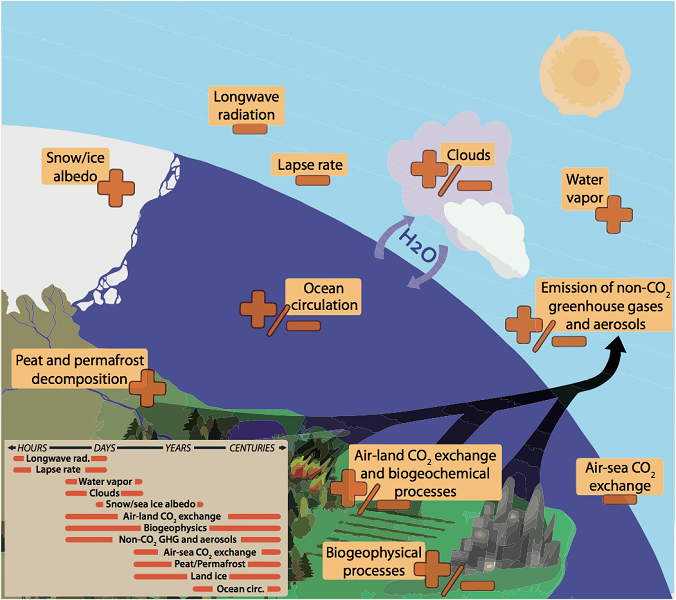
However, the multitude of processes and components that together form the climate system results in phenomena of amplification and damping of the climate system’s response to forcings. A well-known example of amplification is related to the presence of snow. As the climate warms, the snow cover recedes. Previously snow-covered and white surfaces become darker. A dark surface reflects solar radiation less well and absorbs it more. This increased absorption of solar radiation warms the surface, which will lead to an increased reduction in snow cover. This is therefore an amplification of climate variation by a process internal to the climate system: it is called a positive reaction. In the case of amortization, this is called negative feedback. It is important to note here that positive feedback does not generally lead to a “runaway” system.

The fact that our climate system has allowed life to develop for billions of years proves that they are generally feedback that amplifies the system’s response by a factor much closer to 1 than 10. However, it should be noted that the combined effect of the main climate feedbacks involved in current climate change is positive. These main feedbacks are related to cloud cover, water vapour, the vertical structure of the atmosphere, and the extent of ice and snow (Figure 4, [2]). The feedback from water vapour is very strong because its concentration adjusts very quickly (~10 days) to atmospheric temperature.

5. Abrupt and irreversible changes

Sometimes, the response of a component of the climate system or the climate itself to a slowly changing external forcing accelerates abruptly: we speak of abrupt changes. The existence of such abrupt changes is often, but not always, linked to positive feedback. It can also mean, in a very simple way, exceeding a physical or biological threshold, for example, melting ice from the moment the temperature reaches 0°C, or the disappearance of an ecosystem when a tolerance threshold (e. g. drought) is exceeded. The rapid evolution of the subsystem concerned can in turn lead to rapid climate change.

The issue of the irreversibility of climate change is linked to the issue of abrupt changes. A change is defined as irreversible if, after cancellation of the initial forcing, the system does not return to its initial state within a period of time of the same order of magnitude as the duration of the cancellation of the forcing. For example, it is currently estimated that prolonged exposure (a few hundred years) of the Greenland ice cap to a climate 2°C warmer than the climate of the early 19^e century (“pre-industrial”) would most likely lead to the near-total melting of this ice cap in a few thousand years. If, once the melting process of the ice cap is well under way, the global climate returns to its original state at the beginning of the 19th century, the ice cap will no longer return to its former configuration: indeed, following a partial melting, the surface of the ice cap will be at a lower altitude and therefore exposed to a warmer climate (it is recalled that the vast land shelf below the Greenland ice cap is currently at an altitude of over 3000 m).

The identification of elements of the climate system that may react abruptly and/or irreversibly and the quantification of the thresholds of change involved are aspects of current climate research.

6. Climatology, a multidisciplinary science

At the beginning of this article, the difference between meteorology and climatology was described as related to time scales, short (on the order of a week) for meteorology and long (beyond the month, with integration periods of several decades) for climatology. We can also see, in more mathematical terms, meteorology as a problem under initial conditions (“Given the state of the atmosphere today, what will be its state in three days? “), while climatology is a problem at boundary conditions (“What will be the average weather in 50 years if I change the concentration of CO₂ in the atmosphere? “»). We can clearly see in this last question the concept of climate system forcings coming back. That being said, climatology is in a sense a daughter of meteorology, and it shares many tools and methods with meteorology (read Introduction to weather forecasting).

Nevertheless, climatology, because it necessarily has to take into account more physical and biological phenomena than meteorology, is a multidisciplinary science: the components of the climate system – biosphere, atmosphere, ocean, ice, continental surfaces – are understood through biology, chemistry, physics, geology, hydrology, and other sciences. Climatological tools, including climate models, make extensive use of applied mathematics (read Biosphere, hydrosphere and cryosphere models).

For obvious reasons, climatology has a crucial need for long-term observations and with good spatial coverage . The work of collecting these data, their processing (homogenization, etc.) and their analysis is colossal, and not very visible to the general public. These are the long series of temperature and precipitation readings, the long series of glacier observations, which are the starting point for almost all climate science. Unlike other sciences, experimentation, on the other hand, is less present, simply because we have only one climate system, one planet, with which we cannot conduct a controlled experiment. That being said, humanity is carrying out a gigantic experiment to artificially increase the concentration of the main long-life greenhouse gases in the atmosphere! However, some details of the climate system may be accessible for experimental quantification: for example, it is possible to experimentally analyze the response of trees to a local and persistent increase in CO₂ concentration in the ambient atmosphere, as was done in the FACE experiments (Free-Air Carbon dioxide Enrichment).

Since the climate system as such is inaccessible to experimentation, the only way to predict its evolution in detail is by modelling based on our current understanding. Given the complexity of the system, detailed mathematical modelling is not possible in an analytical way. The number of processes involved is far too large, so it is necessary to switch to numerical modelling. This involves representing the physical, chemical and biological processes involved in as detailed a manner as possible, in the form of equations transformed into computer code in order to calculate the evolution of the system using powerful computers. The most comprehensive tools often used for century scale climate projections are the Coupled Earth System Models. They represent the detailed and coupled functioning of the essential subsystems of the climate system. To do this, the atmosphere is represented, for example, by a mesh size of about 100 km horizontally and about 50 vertical levels. The evolution of the state of the atmosphere is then calculated over several decades with a time step of a few minutes from a given initial state. The computer thus simulates the weather in all parts of the world (with a resolution of about 100 kilometres), step by step. So it is literally “the rain and the sun”. The processes represented are terrestrial fluid dynamics, which governs the movement of air masses, radiative transfer, small-scale turbulence processes, cloud formation, precipitation, etc. The computer calculates in the same way the evolution of the ocean and the other components of the climate system as well as their exchanges of water, energy, carbon, etc., in essentially the same time step. Because of the complexity of the climate system, these coupled models of the Earth system are among the largest consumers of computing power in the world.

The collection and interpretation of past climate indicators (ocean sediments, ice cores, etc.) is a particular branch of climatology, namely palaeoclimatology. Knowledge of past climate change provides an extremely valuable perspective on current climate change. It also allows us to test our understanding of the climate system and our climate models in a different context than the current one, and thus to assess the robustness and validity of our understanding and models.

 

---

References and notes

[1] Store, T.F., D. Qin, G.-K. Plattner, L.V. Alexander, et al., 2013. Technical summary. In: Climate Change 2013: The Science. Contribution of Working Group I to the Fifth Assessment Report of the Intergovernmental Panel on Climate Change[Stocker, T.F., D. Qin, G.-K. Plattner, M. Tignor, S.K. Allen, J. Boschung, A. Nauels, Y. Xia, V. Bex and P.M. Midgley (eds.)]. Cambridge University Press, Cambridge, United Kingdom and New York (NY), United States of America. https://www.ipcc.ch/pdf/assessment-report/ar5/wg1/WG1AR5_SPM_brochure_fr.pdf

[2] Cubasch, U., D. Wuebbles, D. Chen, M.C. Facchini, D. Frame, N. Mahowald and J.-G. Winther, 2013. Introduction. In: Climate Change 2013: The Physical Science Basis. Contribution of Working Group I to the Fifth Assessment Report of the Intergovernmental Panel on Climate Change[Stocker, T.F., D. Qin, G.-K. Plattner, M. Tignor, S.K. Allen, J. Boschung, A. Nauels, Y. Xia, V. Bex and P.M. Midgley (eds.)]. Cambridge University Press, Cambridge, United Kingdom and New York, NY, USA, pp. 119-158, doi:10.1017/CBO9781107415324.007. https://www.ipcc.ch/pdf/assessment-report/ar5/wg1/WG1AR5_Chapter01_FINAL.pdf