The seasonal forecast
PDF
This article shows how the numerical models used for numerical weather prediction can be used to provide information on the weather over the next few months, despite their limitations. It presents how scientists have organized themselves to give an operational status to this activity, which still remains a research activity, although it has already conquered some applications.
1. Why a season-wide forecast?
Weather forecasting is based on the resolution by a computer of fluid mechanics equations from observations of the atmosphere-ocean-cryosphere system-continental surfaces (see Introduction to weather forecasting). Thus, from the observation of the D-day, we can describe with some precision the state of the D+1-day. By a simple reasoning, we deduce that the state of the day D+2 is accessible by the same process, then the day D+3… We could believe that there is no limit to the possibility of producing forecasts, except for the calculation resource. In practical terms, it was quickly realized that the quality of the forecasts decreased very quickly with time: after a few days (about a week in 2016) a forecasted weather situation does not look any more like the actual situation than a situation taken at random in the same month in previous years. Lorenz (1963) [1] showed that even if the weather models were perfect, a very small error in describing the initial conditions made it impossible to forecast beyond an estimated limit of 10-15 days for the atmosphere. This notion has been popularized by the term butterfly effect.
It is therefore not possible to make deterministic forecasts at the season level. However, there are phenomena in nature whose evolution over a few months is not chaotic (see section 3) and which influence the behaviour of the atmosphere. And, moreover, there is a real need for long-term forecasts in many human, agricultural, industrial or tourist activities. If we have numerical models that faithfully simulate the evolution of these slow phenomena, and that are able to reproduce on average the effect of these phenomena on the perceived time (i.e. temperature, wind, rain, etc.), then we can hope to provide partial information on what will happen in the coming months.
A distinction is made between the monthly forecast, which aims to describe even a rough chronology (for example, a hot episode at the end of January), and the seasonal forecast, which abandons any chronological approach to describe a season in purely statistical terms (for example, a significant probability of having a cold episode next winter). In 2016 monthly forecasts are generally produced until month M+2; seasonal forecasts are generally produced until month M+7 (see section 4). In the following, we will describe how these seasonal forecasts are produced and what can be expected from them.
2. Yes, but how do we make these forecasts?
Seasonal forecasting is the heir to weather forecasting through the numerical tools it uses. However, it took more than thirty years between the first operational short-term forecasts and the first seasonal forecasts (Palmer and Anderson, 1994) [2]. Indeed, three particularly difficult technical steps had to be taken:
- early 1980s: emergence of atmospheric models and daily observations covering the entire globe,
- early 1990s: emergence of coupled ocean-atmosphere models whose behaviour on the globe is reasonably similar to observations, when considering an average over several decades,
- early 2000s: establishment of a three-dimensional Argo global ocean observation network [3].
We sometimes talk about seamless forecasting for the production of forecasts at 24h, 10 days, one month, 6 months, 6 months, 10 years, or even climate scenarios for the end of the century. This expression underlines the need to share scientific and technological developments. Thus, the model used in Météo-France for seasonal forecasting is also the one used for the IPCC (International Panel on Climate Change) climate scenarios and its component for the atmosphere and continental surfaces is the model used by Météo-France for short-term weather forecasting.
For practical reasons, there are implementation differences between the seasonal forecast and the short-term forecast:
- Accurate modelling and initialization of the ocean, a slow component of the system, is essential for seasonal maturity. It is only justified for a few applications after 2-3 days.
- The forecast we are trying to make at the seasonal maturity is not of a deterministic nature but of a statistical nature. It is therefore necessary to make at least 50 forecasts to obtain robust statistical estimates. We talk about ensemble forecasting (see The Ensemble forecasting).
- In the short term, the main source of uncertainty concerns the initial state. At the seasonal scale, it is also necessary to take into account the differences between the simulated climate and the actual climate.
3. A forecast is true!
The difficulty of assessing a seasonal forecast has long delayed the consensus on the validity of a scientific approach.
In short-term forecasting, the success and failure rate of a forecasting system can be assessed after a few months. In seasonal forecasting, it would take decades to make a reliable judgment. Therefore, we look to the past by producing what are called re-forecasts. A re-forecast is a forecast produced retrospectively, years later, but without cheating, i.e. by not using any information after the initial time of the forecast. These re-forecasts should cover both a long period (for statistical reasons) and a recent period (for reasons of homogeneity of the observation system). Operational applications start this period in 1993 (satellite altimetry observation begins), while research mode evaluations begin in 1979 (satellite global ocean temperature observation begins). Producing a set of re-forecasts covering the last 30 or 40 years takes from six months to one year. This waiting time protects the researcher from the bias of choosing the best system from among a large number, based on the highest success rate. This success rate is generally measured by an index called the forecast score. A score is a number generally between 0 and 1, corresponding to a trivial forecast, for example systematically predicting the climatology of the month and place, 1 corresponding to a perfect forecast. A forecast can have a negative score, for example when it systematically announces the opposite of what is observed. A very often used score is the correlation coefficient between two time series. This index between -1 and 1 is 0 if the series are independent, and 1 if one can move from one to the other by an increasing linear algebraic relationship. Its precise definition is based on the second order moments of the statistical distribution (Jolliffe and Stephenson, 2012 [4]).
The notion of mild or cold winter has only a statistical reality at our latitudes. During the same winter, there are a succession of hot and cold episodes. Sometimes the latter are more numerous or more intense. With sets of 50 daily forecast members, a predicted probability law can be reconstructed. Estimating a probability for observations in a given winter is much more difficult, as only 90 values are available, and these values are not independent because there is some persistence from one day to the next… The evaluation by a correlation coefficient is insufficient because it does not take into account the uncertainty inherent in a non-deterministic forecast. The probabilistic assessment is more delicate because the phenomenon to be predicted (the probability of a cold wave) can only be estimated roughly. Many probabilistic scores are available (Jolliffe and Stephenson, 2012 [4]). If they are of interest to the researcher, they are difficult to compare between models because there is no consensus on a single score.
For a more reliable assessment, we turn to slow-moving phenomena that maintain a constant characteristic over the course of a season, while offering a high degree of variability from one year to the next. There are three of them that are accessible to both observation and modelling, and for which satisfactory scores are now available.
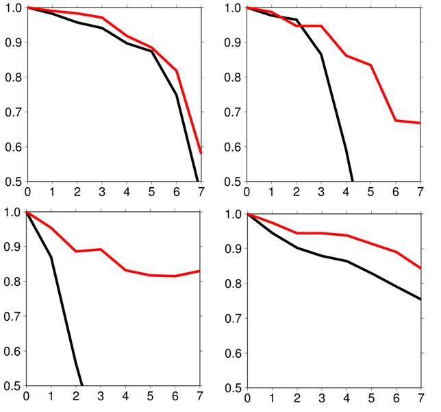
- A well-known phenomenon since the 1980s (Shukla 1981) [5], the surface temperature of the equatorial Pacific Ocean: as shown in Figure 1, the ENSO phenomenon (El Niño Southern Oscilation) offers remarkable predictability up to 7 months (red curve); in winter and autumn, the phenomenon is very persistent (black curve), but the model does as well or better.
- Phenomenon discovered quite recently: the extent of Arctic ice pack (Chevallier et al., 2013) [6].
- Less useful in practice, but scientifically interesting: wind in the equatorial stratosphere (Boer and Hamilton, 2008) [7].
Nevertheless, it is necessary to estimate predictability at mid-latitudes, even if it is low. The usual measure of the quality of this type of forecast is the correlation coefficient (mentioned above) between the expected seasonal average and the observed average, which has the advantage of being used for a long time and being universally used, even if it is not very robust over 30-year series and does not take into account the dispersion of the forecast set.
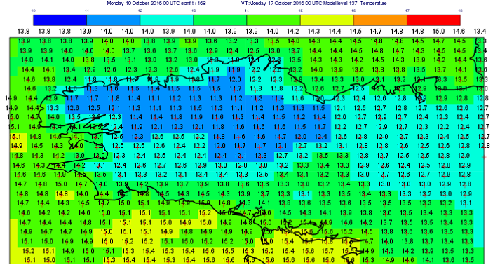
Figure 2 shows the values of this coefficient for the four-season temperature forecasts (DJF, MAM, JJA, SON, where each capital letter is the initial of a month of the year) for the temperature over Europe. The trend due to global warming has been subtracted because it artificially inflates the scores.

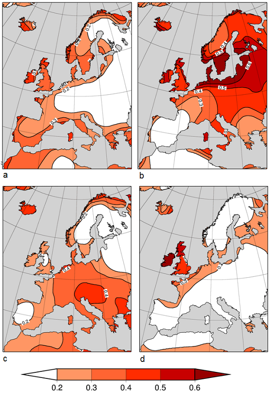
A coefficient of less than 0.2 is considered to provide no usable information. It can be seen that predictability varies from region to region and from season to season. In winter (Figure 2a) the oceanic façade is favoured. In summer (Figure 2c), the Southeast of the continent is the preferred region. Figure 3 shows the same scores, but for a forecast by persistence of the initial situation. It can be seen that in the shoulder seasons this low-cost method of calculation generally does better than the model. A lesson in modesty!
4. The operational implementation of the forecasts
In Section 2, it was written that systematic model defects were a source of both error (which can be corrected a posteriori) and uncertainty (which must be estimated). This implies producing not only forecasts, but also re-forecasts (this term has been defined in section 3). In a research activity, we only carry out re-forecasts.
Operational forecasts consist of comparing an average of expected situations with a multi-year average called the reference climate. For this purpose, we have a set of re-estimates of past years. This game is also used to estimate the expected scores for the forecast. It is essential to have perfect homogeneity between re-forecasts and forecasting. This means that the two productions differ only in the initial condition. There is no question of making any changes in the model between the re-forecasts, made once and for all, and the forecast made each month. Given the time required to carry out a re-forecast (six months to one year), the forecast centres only change versions every two or three years.
To estimate the uncertainty associated with model imperfections, the most commonly used method is the multi-model approach. Indeed, each model is built on the basis of choices and hypotheses that are specific to the centre that implements it. Sometimes the forecasts of two models disagree. For example, there are consortia in Europe (Eurosip), North America (NMME) and Asia (APCC) that combine forecasts from several models. These forecasts are available free of charge in the form of maps or bulletins. In the USA and soon in Europe (Copernicus Climate Change Service programme of the European Union) digital data are freely accessible every month for the next six months.
5. What is the purpose of seasonal forecasts?
Seasonal forecasts are essentially made to be distributed to all potential users in the form of maps or bulletins via the web (European Medium-Term Forecast Centre [8] Météo-France [9]). The consequences of a hot event in the equatorial Pacific (El Niño) are sufficiently documented [10] for a prediction of its occurrence to be interpreted in terms of droughts, fisheries resources, flood risk..
There are also seasonal forecast applications developed for specific use. It is especially in tropical regions, where scores are higher, that there is collaboration between forecasters and users, usually through statistical adaptation. This type of approach requires re-forecasts over long periods of time and infrequent version changes. For example, the management of a dam on the Senegal River includes a seasonal forecast component (Bader et al., 2006 [11]). In South America, a number of statistical adaptations are being made by the Eurobrisa consortium [12].
In Europe, users are often discouraged by low scores (Bruno-Soares and Dessai, 2016 [13]). In France, studies have been carried out on wheat yield (Canal, 2014 [14]) or on river flow and soil moisture (Singla et al., 2012 [15]). This last application is now operational. Prototypes are being developed in Europe in other fields of application, through the Euporias project [16] : impact of winter conditions on transport in the United Kingdom, renewable energy production in Spain, hydropower management in Sweden.
6. What future for seasonal forecasts?
With an ambitious objective and strongly limited by the constraints of physics (butterfly effect) and technology (digital computer resources), seasonal forecasting often disappoints at first glance. However, its additional cost compared to a weather forecasting system is very low and the services it can provide are undeniable if you accept risk management. Progress on the quality of forecasts is visible if we compare the state of the art in 2015 with that of 2005 or 1995, but very little progress is made from one year to the next, which sometimes gives a false idea of stagnation.
The most predictable advances will come from the increase in horizontal and vertical resolution of the models and the complexity of the representation of heat and humidity sources (known as physical parameterizations). Indeed, this effort is common to that on improving weather forecasting and climate modelling. But there are also more specific research axes such as the introduction of perturbations in the equations to simulate model errors (Batté and Doblas-Reyes, 2015 [17]), or as the statistical post-processing of forecasts taking into account model errors over a learning period. Slowly changing parameters such as snow cover or soil moisture play a role in the system’s seasonal scale memory. The refinement of their initialization in forecasts and re-forecasts is also a potential source of improvement.
References and notes
[1] Lorenz (1963). Deterministic nonperiodic flow. Journal of Atmospheric Sciences,20, 130-141.
[2] Palmer, T.N. and Anderson, D.L.T. (1994). The prospects for seasonal forecasting – a review paper”. Quarterly Journal of the Royal Meteorological Society, 120, 755-793.
[3] ARGO. Part of the integrated observation strategy.
[4] Jolliffe IT and Stephenson DB (2012) Forecast Verification. 2nd edition, Chichester (UK), Wiley-Blackwell
[5] Shukla J. (1981) Dynamical predictability of monthly means. Journal of Atmospheric Sciences, 38″,2547-2572.
[6] Chevallier M., Salas y Mélia D., Voldoire A., Déqué M. and Garric G. (2013). Seasonal Forecasts of the Pan-Arctic Sea Ice Extent Using a GCM-Based Seasonal Prediction System. Journal of Climate, 26, 6092-6104.
[7] Boer G.J. and Hamilton K. (2008). QBO influence on extratropical predictive skill. Climate Dynamics, 31, 987-1000.
[9] Météo-France, Seasonal forecast (public site, but identification required),
[10] Météo-France, Understanding: El Nino and La Nina
[11] Bader JC, Piedelievre JP, and Lamagat JP (2006). Seasonal forecast of the Senegal River flood volume: use of the results of the ARPEGE Climat model. Hydrological Science Journal, 51:3, 406-417, DOI: 10.1623/hysj.51.3.406
[12] Eurobrisa; A EURO-BRazilian Initiative for improving South American seasonal forecasts.
[13] Bruno Soares M and Dessai, S. (2016). Barriers and enablers to the use of seasonal climate forecasts amongst organisations in Europe. Climatic Change, 1-2, 89-103. DOI: 10.1007/s10584
[14] Channel N, (2014). Application of seasonal forecasting to agriculture: assessment at the scale of France. Thesis from the University Paul Sabatier. Toulouse
[15] inla S, Ceron JP, Martin E, Regimbeau F, Déqué M, Habets F and Vidal JP (2012). Predictability of soil moisture and river ows over France for the spring season. Hydrology and Earth System Sciences, 16, 201-216.
[16] Euporias. European Provision Of Regional Impacts Assessments on Seasonal and Decadal Timescales.
[17] Batté L. and Doblas-Reyes F.J. (2015) Stochastic atmospheric perturbations in the EC-Earth3 earth system model: impact of SPPT on seasonal forecast quality. Climate Dynamics, 45, 3419-3439.
The Encyclopedia of the Environment by the Association des Encyclopédies de l'Environnement et de l'Énergie (www.a3e.fr), contractually linked to the University of Grenoble Alpes and Grenoble INP, and sponsored by the French Academy of Sciences.
To cite this article: DEQUE Michel (January 5, 2025), The seasonal forecast, Encyclopedia of the Environment, Accessed July 13, 2026 [online ISSN 2555-0950] url : https://www.encyclopedie-environnement.org/en/air-en/seasonal-forecast-2/.
The articles in the Encyclopedia of the Environment are made available under the terms of the Creative Commons BY-NC-SA license, which authorizes reproduction subject to: citing the source, not making commercial use of them, sharing identical initial conditions, reproducing at each reuse or distribution the mention of this Creative Commons BY-NC-SA license.