


地球平均温度

全球气候变化是一个重要的问题。基于科学界的声明,人类活动是造成当前以及未来全球变暖的原因。但是,我们真的能够确定地球平均温度吗?如果能,又该如何测量它?当我们给出上个世纪的变暖趋势,或者当国际社会设定将全球温升控制在2℃甚至1.5℃的目标时,我们的测量真的能精确到零点几摄氏度吗?在此,我们讨论了确定地球表面平均温度的方法问题、当前重建的准确性以及最近演变的观测和原因等问题。
1.全球平均温度意义何在?
1.1能量平衡与全球温度的关系
[图片来源:怀尔德(Wild)等,2015 [1]]
气候系统(包括大气、海洋、冰盖、植被等)接收的能量大部分来自太阳(图1)[1]。这些以辐射形式接收的能量大致相当于温度为5800 K的黑体(参见:“黑体热辐射”)在可见光区的辐射量。在透过大气层时,部分辐射被反射或被云层、空气中的颗粒(气溶胶)和大气气体所散射。另一部分辐射被这些气体和气溶胶所吸收。只有部分太阳辐射能够到达地表,在地表它也被部分反射。因此,入射到大气层顶部的太阳辐射(340 W/m2)只有大约一半被地球表面吸收(160 W/m2)。
海洋和陆地获得的能量输入被等量的能量损耗所抵消,从而达到能量平衡。损耗的形式可以是辐射能,或是与传导有关的热量转移(称作显热),也可以是和水相变有关的热量转移(称作潜热)。这些能量损耗都是地球温度的函数,特别是地表辐射,它接近于288 K的黑体辐射,因此属于红外光范围。
地球温度在不断发生变化,从而使地表和大气层顶部能量趋于平衡。但是,即使这个物理机制是众所周知的,全球平均温度的概念依然不容易掌握。
1.2.平均温度?一个统计指标!
固体、液体或气体介质的温度是反映特定环境下构成该介质的粒子运动的物理量,所以把两个温度相加不具有物理意义。因此,对各地不同且跨度很大的温度进行平均计算没有直接的物理解释。地表平均温度正是如此,它涵盖了温暖的热带地区和寒冷的极地地区。然而,平均温度是一个统计指标,并且已被证明非常有助于评估过去以及未来几个世纪全球范围内的气候变化。全球平均温度反映的气候变化可以用可识别的潜在物理机制来解释。
1.3.举例一: 温室气体对地球平均温度的影响
第一个例子是平均温差,可以通过计算由于大气中自然产生的温室气体的存在而产生的地球能量平衡来估计。这些气体具有吸收地球表面发出的红外辐射的特性,然后将其中一些重新发射回地球表面,从而进一步使地球变暖(图1)。主要的温室气体包括水蒸气、二氧化碳(CO2)、甲烷(CH4)。温室气体对全球平均温度的影响之一是33 ℃的升温效应,可以将全球平均温度从-18℃提升至15℃。
应该注意的是,这种计算方法只有在“所有条件都相同”的情况下才有意义,因为如果地球温度降低约30度,由于太阳辐射的反射增加(冰-反射率反馈效应)地表冰盖变化将导致额外的冷却。
1.4. 举例二: 地球轨道参数对平均温度的影响
物理过程导致地球平均温度出现较大偏差的另一个例子,主要是由地球轨道偏心率的变化引起的。地球绕太阳公转的轨道是一个椭圆,其偏心率,即测量形状与圆形之间的偏差,在过去一百万年里在0(圆形轨道)和0.06之间变化,主周期约为10万年。随着偏心率增加,地球到太阳的平均距离也会增加,因此地球接收的太阳辐射能减少。其结果是,在过去大约一百万年的时间里,形成了一个10万年寒冷(冰川期)和温暖(间冰期)交替的气候循环。
对10万年周期的理解仍在研究中,因为地球接收的能量变化的直接影响很小。一些研究表明[2],其他天文参数变化的影响(倾角、岁差;参见:“环境自然演变的动力”)以及那些放大寒热期温差的物理效应也应该被考虑:
前面提到的冰-反射率反馈效应:暖期冰盖减少,降低了太阳辐射在地球表面的反射率(反照率),地表吸收的辐射能增加,从而加剧变暖。
温室效应:在温暖期,温室气体浓度也会受物理过程和生态系统变化影响而增加。
因此,约21000年前最后一个极端寒冷时期(末次冰期冰盛期,LGM)和我们已知的大约10000年前温暖间冰期之间的全球平均温差可能在3到8摄氏度之间[3]。
动画“气候变化的驱动力”[致谢:图卢兹博物馆(Museum de Toulouse),墨卡托海洋国际公司(Mercator Océan )]
1.5.总结
因此,全球平均温度必须被视为地球表面气候演变的一个统计指标。上述两个例子表明,这一指标在多大程度上能够灵敏地反映地球气候平衡中涉及的物理和生物过程,尤其是那些对能量平衡有影响的过程。
此外,第二个例子与已观测到的地球气候变化相符,表明该指标的几度偏差可以带来非常显著的气候变化。末次盛冰期温度降低几度意味着北半球冰盖覆盖范围的扩大(比如覆盖不列颠群岛北部)以及海平面下降约130米。
2.基于仪器数据的全球平均温度重建
2.1.地表观测
(参考 Ground Weather Observations: What are we measuring and what do we do with them?)
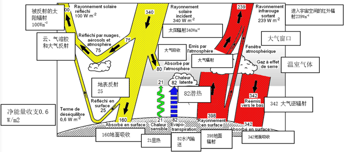
[图片来源:公有领域]
评估全球平均温度是一个挑战。由于不同地区之间的温度变化显著,测定的准确度取决于地表观测手段。研究平均温度随时间的变化还需要进行一系列统一、不间断的测量,测量方式要能克服干扰,尤其是克服传感器或者测量环境变化造成的干扰。
海洋[4]和陆地[5]仪器观测始于17世纪,1856年出现了第一个气象观测网络。该网络在法国天文学家奥本·勒威耶(Urbain Le Verrier)[6]的指导下,由巴黎天文台的埃马纽埃尔·利亚斯(Emmanuel Liais)管理。因此,基于温度计测量的全球平均温度重建工作最早可以追溯到1850年。
一些研究团队也开展了基于温度估算的间接重建工作。该工作利用的是自然档案(如冰芯、沉积物、树木年轮、珊瑚……)和数据模型。间接重建虽然覆盖的时间更长,但在准确度和全球覆盖率上还未达到仪器重建的水平。
2.2.数据源
19世纪后半叶,主要有三个团队开始着手进行全球平均温度重建,包括美国国家航空航天局戈达德空间科学研究所(NASA Goddard Institute for Space Science)[7]、美国国家海洋和大气管理局(National Oceanic and Atmospheric Administration, NOAA)[8]、以及来自英国气象局哈德利中心(UK Met-Office)和东安格利亚大学气候研究室(Climate Research Unit of the University of East Anglia)[9]的英国团队。
这三个重建工作中的部分源数据是相通的,大部分数据也是可获取的:
陆地区域的数据来自全球历史气候网(Global Historical Climatology Network, GHCN)[10],这些数据来自美国国家航空航天局(NASA)和NOAA为最新版本(GHCNv4)重建的约25000个站点对遮蔽空气温度的观测(图2)。
海洋区域的数据来自国际海洋大气综合数据集(International Comprehensive Ocean-Atmosphere Data Set, ICOADS)[4]。
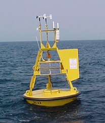
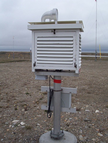
[图片来源: 公有领域]
美国重建主要使用的是GHCN数据,而英国重建除了使用了部分GHCN数据,还使用了直接从国家气象部门或者其他国际气候数据库获得的数据[11]。另一方面,这三种重建基本上都是基于ICOADS的海洋数据。
陆地温度数据是在地表附近的空气中测量的,世界气象组织(参见:“地表气象观测:测量什么以及如何测量”)建议的测量高度在1.25米到2米之间(法国为1.5米)。然而,相比于水温测量,在船上或者浮标上测量空气温度没有那么准确,主要原因在于传感器会被盐污染,而且在船上难以测量海面以上高度的温度。因此重建者通常选择在水中而非空气中测量海面温度(图3)。只要每个重建过程的计算方法一致,这种测量方法就不会影响全球平均温度变化的研究。但是,在估算不确定性时,必须要考虑方法差异带来的影响(参见2.4)。
全球平均温度的重建取决于档案文件中以往观测数据的收集和保存。因此,随着诸如在国际I-DARE项目框架内的收集的数据被重新处理,数据的时间和空间覆盖面有望在未来得到完善,特别是在历史最久远的时期[12]。
2.3.平均值计算方法
由于数据在空间上是分散的,在重建的早期阶段,一些区域的数据覆盖率比较低。另一方面,一些观测可能集中在某些地区,例如欧洲大陆和北大西洋。因此,有必要采用兼顾空间异质性的平均化程序。计算程序因不同的重建而不同,由于计算程序在科学文献出版物中已有准确记录,在此只作概述。
在英国的重建工作中,现有的观测数据是在5°经度乘以5°纬度的网格上取平均值,无需任何插值,然后按相应区域计算加权平均,获得全球平均值[9]。对于NASA来说,大陆重建主要的中间步骤还包括在地面网格内求平均值(面积相同的8000个网格),但是在1200千米半径内按每个网格中心的距离加权[7]。NOAA的大陆重建更复杂,因为它涉及到考虑观测间空间关系的统计函数(Empirical Orthogonal Teleconnection Functions or EOTs),对数据进行插值(和外推)。这些函数的影响范围限于每个网格中心周围2000km(纬度)×4000km(经度)的区域[8]。美国重建正是使用这些函数在2°(经度)×2°(纬度)的网格内对海面温度数据插值、外推。在这种情况下,EOT的空间影响范围被限制在每个网格中心和周围3000千米(纬度)×5000千米(经度)的区域[13]。
世界气象组织建议计算30年内气候平均值(气候学)的偏移或者异常值。虽然三组重建选择的基准期不同(英国团队和NOAA选择1961~1990年;NASA选择了1951~1980年),但这对最终结果没有任何影响,因为在重建过程中只关注温度的时间变化而非难以阐释的温度绝对值。这样可以在给定网格中测平均温度时,不受站点的海拔差异影响。
重建工作是在覆盖地球的网格上进行的(NOAA[14]使用5°×5°的网格,英国[15]和NASA重建使用2°×2°的网格[16])。通过重建,不仅可以计算全球平均值,还能绘制不同区域的温度趋势图。从1850年开始,英国的重建工作按月和按年进行,而NASA和NOAA则是从1880年开始进行重建的。
2.4.误差估计和修正
[图片来源: 政府间气候变化专门委员会(IPCC) 2013 [3]]
科研论文和IPCC(政府间气候变化专门委员会)陆续发布的报告都分析了全球平均温度重建的误差来源,而且分析了用于纠正误差的方法。在此,我们只讨论误差产生的主要原因,这些原因在“误差计算”有详细说明。有些与取样(每个计算网格单元的观测数量)和不完全覆盖(一些网格单元没有观测;图4)有关。地面观测站周围城镇化的影响导致了人为的变暖趋势,这也是我们需要考虑的因素。由于观测站、仪器、气象站位置的变化或其他任何可能影响测量的变化破坏了系列数据的一致性,这点应在重建修正和相关误差估计中予以考虑。因为所使用的观测手段变化,海洋数据也应进行偏差的修正。
全球范围内,无论是在海洋或者大陆,全球年平均温度的不确定性是通过综合所有可以估计的误差或者不确定性来计算的。通过NASA[8]、NOAA[9]和英国团队[9]提出的重建,最终得到了对平均温度的各种估计。尽管使用的方法不同,但各重建的估计值都非常接近。NOAA重建和其他两种重建之间的主要区别在于取样和空间覆盖误差。前者先验地更好地考虑了20世纪中叶以来的北极数据,从而降低了不确定性。
3.过去的两个世纪全球平均温度是如何变化的,以及为何变化?
3.1.趋势探究
图5摘自世界气象组织(World Meteorological Organization)年度报告[17]。该图显示了根据第二节介绍的三个重建工作获得的1850年至2019年全球平均温度的演变。每个重建工作都要去除1981-2010年的平均值来计算温度值,然后与所谓的“工业化前”参考值(1850-1900年期间的HadCRUT4平均值[9])进行对比。其他两个全球平均温度估算是通过数据再分析得出的(JRA-55数据来自日本气象厅[18],ERA5数据来自欧洲中期天气预报中心[19]),估算结果按照相同的步骤也显示在了图中。(参见:“通过再分析估算地表温度”)
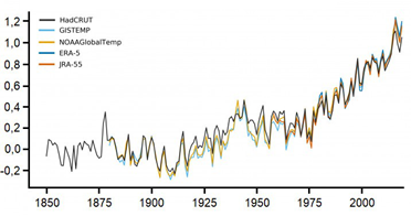
[图片来源:世界气象组织关于2019(2020)年全球气候状况的声明;WMO Pub No.1248.17]
如图5所示,三个重建和两个再分析所得出的温度变化高度一致。其间的差异也与各个重建的总不确定性完全吻合。特别是Huang等人[8]认为,英国和NOAA的重建每年都落在NOAA重建的置信区间内(图13)。主要差异首先来自对1920-1960年间海洋测量偏差的修正处理[7], [9](2.3节)。其次来自于观测数据的空间覆盖以及低覆盖率地区的处理方式不同。特别是NASA和NOAA的重建考虑了北极地区的数据[7]。这样做的效果是更好地再现了这些地区在过去几十年里变暖增加,并导致全球平均温度的上升速度略快于再分析中观察到的结果。
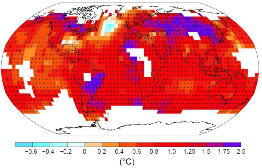
图5还强调了不同时间尺度变异性的叠加。三个重建工作计算出的最长公周期的温度变化趋势都非常接近,并且清楚地表明变暖的程度远远大于每次重建的不确定性。最新的IPCC评估报告[8]包括了对这些趋势的预估和截至2012年计算结果的不确定性。报告中指出,全球平均地表温度在1880~2012年间增加了约0.9℃(90%的概率升温在0.65~1.06℃之间)。为了更好地测量这种变暖,将其与末次盛冰期(约21000年前)和当前时期间的3-8℃的变暖联系起来就足够了(参见第1节)。自IPCC报告发布以来,这种变暖趋势仍在继续,NASA和NOAA估计温升幅度为0.96°C(根据[7],升温幅度有95%的可能在0.81°C~1.11°C)。
3.2.观测到变暖的原因是什么?
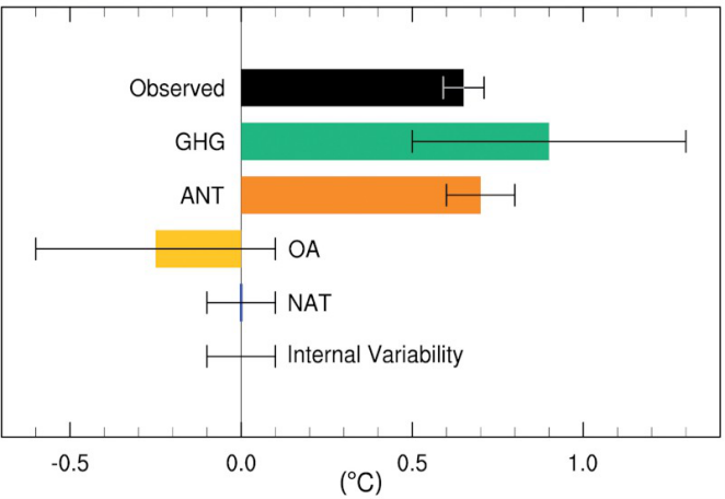
自IPCC于1990年发布第一个报告以来,将变暖全部或部分归因于人类活动所排放的温室气体的问题一直在提出。然而,尽管当时已经观测到了变暖现象和大气中温室气体尤其是二氧化碳浓度增加,但是没有证据证明人为排放的温室气体和变暖的联系,报告在归因上没有给出任何结论。随着研究的不断增加,通过改变可能影响温度的因素来模拟上个世纪的气候—自然因素与太阳变化、火山活动以及气候系统内的变化,或人为的温室气体排放和大气颗粒物(气溶胶)的产生,这些研究提供了大量证据。IPCC连续发布的报告在变暖归因问题上越来越明确。最新的报告[3]得出结论:人为因素极有可能是20世纪中期以来全球变暖现象的主要原因。
图6再现了1951-2010年期间不同因素对温度的变化趋势的贡献估计,并与观测到的趋势进行比较。图6强调了自然因素不是变暖的主要原因,人为因素与变暖现象联系更密切。产生的温室气体(“GHG”)和气溶胶颗粒(“OA”)各自的影响很难准确估算,正如这些估计值周围的“误差棒”所示。
3.3.如何解释数十年的温度变动性?
[图片来源:WMO 2018 [21]]
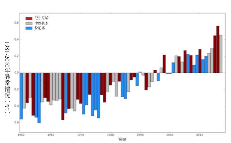
因此,在大约60年时间尺度上清楚地证明了人类活动的影响。然而,在这段时间内,变暖没有规律,因此,在更短的时间跨度内评估人为因素的影响要困难得多。这可以通过图5和图7所示的数十年尺度(几十年)的数据变化来解释,图7通过综合三个重建和两个再分析(2018年版)数据,集中体现了1950-2017年间的情况。
第一个典型的阶段是50到70年代,其特点是:尽管大气中温室气体的浓度增加,但平均温度相对稳定。在短时间内,将人为因素与其他因素的影响区分开来仍然是一个挑战。然而,应当指出,有几项研究表明了另一种人为效应的潜在作用,即大气中气溶胶颗粒浓度的增加,这可能导致在地球表面测得的太阳辐射减少(全球变暗)。因此,从20世纪70年代末以来气温的迅速上升可以部分地解释为工业化国家为限制硫酸盐和碳质颗粒的排放而采取的措施的影响,这些措施也伴随着地表太阳辐射的增加(全球变亮)[20][3]。
另一个导致变暖趋势减弱的多年际变率的例子发生在1998-2012年间。在这段时期,根据HadCRUT4的重建,温度只升高了0.06°C[3]。在这一时期,海平面上升和海洋热含量的增加没有表现出减缓的趋势。近年来,地表变暖减缓的根源是许多出版物的主题,其精确地阐释这个根源依旧是科学争论的焦点(参见:“回顾1998-2013变暖趋势的减缓”)。
最后,图7还显示了温度的年际变化,这也叠加了期趋势上[21]。虽然评估所有因素对既定年温度的影响是不可能的,但可以确定一个重要的自然因素,即热带太平洋区域的暖现象(厄尔尼诺)或冷现象(拉尼娜)。这些现象是海洋和大气相互作用的结果,在几个月时间内改变了海洋表面温度,如图7所示,还对全球平均温度产生了显著的和类似的影响。
4.要记住的信息
地球表面平均温度正在发生变化,以便在它接受的能量和失去的能量之间的达到平衡。
全球平均温度是一个统计指标,对评估全球气候变化尤其重要。
从1850年起,可以使用来自大陆表面空气温度和海洋表面水温观测的仪器数据,按月或年逐级重建。
越来越复杂的不确定性模型使得在其估计中解释各种误差来源成为可能。
根据IPCC的数据,在1880-2012年间,全球平均气温上升了0.9℃,这一变暖幅度远远超过了数据估算的不确定性。
人类活动的影响极有可能是自20世纪中期以来观察到的变暖现象的主要原因。
然而,目前还不太可能准确地量化自然或人为因素在短时间尺度上对平均温度演变的影响程度。
参考资料及说明
封面图片:考虑到纬度和季节带来的已知变动性,我们该如何计算地球平均温度? [图片来源: Pixabay, 无版权图片]
[1] Wild, M., Folini, D., Hakuba, M.Z., Schär, C., Seneviratne, S., Kato, S., Rutan, D., Ammann, C., Wood, E.F., König-Langlo, G. (2015) The energy balance overland and oceans: an assessment based on direct observations and CMIP5 climate models.
[2] Abe-Ouchi, A., Saito, F., Kawamura, K., Raymo, M.E., Okuno, J., Takahashi, K., Blatter, H. (2013) Insolation-driven 100,000-year glacial cycles and hysteresis of ice-sheet volume. Nature, 500, 190-193, DOI :10.1038/nature12374.
[3] Climate Change (2013) The Physical Science Basis Contribution of Working Group I to the Fifth Assessment Report of the Intergovernmental Panel on Climate Change Stocker, T.F., D. Qin, G.-K. Plattner, M. Tignor, S.K. Allen, J. Boschung, A. Nauels, Y. Xia, V. Bex and P.M. Midgley (eds.)]. Cambridge, United Kingdom and New York, NY, USA: Cambridge University Press, 1535 pp. Available at: http://www.ipcc.ch/report/ar5/wg1/
[4] Woodruff, S. D., Worley, S. J., Lubker, S. J., Ji, Z., Freeman, J. E., Berry, D. I., Brohan, P., Kent, E. C., Reynolds, R. W., Smith, S. R., Wilkinson, C. (2011) ICOADS Release 2.5: Extensions and enhancements to the surface marine meteorological archive. International Journal of Climatology, 31, 951-967, DOI: 10.1002/joc.2103.
[5] Rousseau, D. (2013) Les moyennes mensuelles de températures à Paris de 1658 à 1675. La Météorologie, 81, 11-22.
[6] Locher, F. (2009) Les météores de la modernité: la dépression, le télégraphe et la prévision savante du temps (1850-1914). Revue d’histoire moderne et contemporaine, 56, 77-103,
www.cairn.info/revue-d-histoire-moderne-et-contemporaine-2009-4-page-77.htm
[7] Lenssen, N., Schmidt, G., Hansen, J., Menne, M., Persin, A., Ruedy, R., Zyss, D. (2019) Improvements in the uncertainty model in the Goddard Institute for Space Studies Surface Temperature (GISTEMP) analysis. Journal of Geophysical Research: Atmospheres, 124, 6307-6326, DOI:10. 1029/2018JD029522.
[8] Huang, B., Menne, M.J., Boyer, T., Freeman, E., Gleason, B.E., Lawrimore, J.H., Liu, C., Rennie, J.J., Schreck, C.J., Sun, F., Vose, R., Williams, C.N., Yin, X., Zhang, H.M. (2020) Uncertainty estimates for sea surface temperature and land surface air temperature in NOAAGlobalTemp version 5. Journal of Climate, 33, 1351-1379. DOI:10.1175/JCLI-D-19-0395.1.
[9] Morice, C. P., Kennedy, J. J., Rayner, N. A.,Jones, P. D. (2012) Quantifying uncertainties in global and regional temperature change using a set of observational estimates: The HadCRUT4 data set. Journal of Geophysical Research, 117, D08101, DOI: 10.1029/2011JD017187.
[10] Lawrimore, J. H., Menne, M. J., Gleason, B. E., Williams, C. N., Wuertz, D. B., Vose, R. S., Rennie, J. (2011) An overview of the Global Historical Climatology Network monthly mean temperature dataset, version 3, Journal of Geophysical Research, 116, D19121, DOI: 10.1029/2011JD016187.
[11] Jones, P.D., Lister, D.H., Osborn, T.J., Harpham, C., Salmon, M., Morice C.P. (2012) Hemispheric and large-scale land surface air temperature variations: An extensive revision and an update to 2010, Journal of Geophysical Research, 117, D05127, DOI: 10.1029/2011JD017139.
[12] I-DARE International Data Rescue Portal The International Data Rescue Assistance Portal (I-DARE). Available at: https://www.idare-portal.org/
[13] Huang, B., Banzon, V.F., Freeman, E., Lawrimore, J., Liu, W., Peterson, T.C., Smith, T.M., Thorne, P.W., Woodruff, S.D., Zhang, H.-M. (2015) Extended Reconstructed Sea Surface Temperature version 4 (ERSST.v4). Part I: Upgrades and intercomparisons. Journal of Climate, 28, 911-930, DOI:10.1175/ JCLI-D-14-00006.1.
[14] https://psl.noaa.gov/data/gridded/data.mlost.html
[15] https://crudata.uea.ac.uk/cru/data/temperature/
[16] GISS Surface Temperature Analysis (GISTEMP v4), NASA.
[17] WMO statement on the state of the global climate in 2019 (2020) WMO Pub No.1248. Geneva: WMO. ISBN: 978-92-62-11248-5.
[18] Japan Meteorological Agency JRA-55 – the Japanese 55-year Reanalysis.
[19] European Centre for Medium-Range Weather Forecasts. ERA5.
[20] Wild, M. (2009) Global dimming and brightening: A review. Journal of Geophysical Research, 114, D00D16. DOI:10.1029/2008JD011470.
[21] World Meteorological Organization. Media – Press Release – World Meteorological Organization confirms that 2017 ranks among the three warmest years on record.
L’Encyclopédie de l’environnement est publiée par l’Université Grenoble Alpes – www.univ-grenoble-alpes.fr
Pour citer cet article: Auteur : PLANTON Serge (2020), The average temperature of the earth, Encyclopédie de l’Environnement, [en ligne ISSN 2555-0950] url : http://www.encyclopedie-environnement.org/?p=11589
Les articles de l’Encyclopédie de l’environnement sont mis à disposition selon les termes de la licence Creative Commons Attribution – Pas d’Utilisation Commerciale – Pas de Modification 4.0 International.
环境百科全书由环境和能源百科全书协会出版 (www.a3e.fr),该协会与格勒诺布尔阿尔卑斯大学和格勒诺布尔INP有合同关系,并由法国科学院赞助。
引用这篇文章: PLANTON Serge (2025年1月5日), 地球平均温度, 环境百科全书,咨询于 2026年7月5日 [在线ISSN 2555-0950]网址: https://www.encyclopedie-environnement.org/zh/climat-zh/average-temperature-earth-2/.
环境百科全书中的文章是根据知识共享BY-NC-SA许可条款提供的,该许可授权复制的条件是:引用来源,不作商业使用,共享相同的初始条件,并且在每次重复使用或分发时复制知识共享BY-NC-SA许可声明。