Assimilation of meteorological data

PDF
Encyclopédie environnement - données météorologique - meterological data

Meteorological observation tools (satellites and ground stations) provide a very large amount of meteorological data, which must be processed to establish the state of the atmosphere from the forecast model. It is this processing that is called data assimilation. It must result in a value of each of the atmosphere parameters in each grid cell of the model. This initial step in weather forecasting is crucial because any initial error has the property of spreading and gradually contaminating the entire atmosphere.

1. The challenge of the starting point for a weather forecast

To predict the weather, major weather centres use a prediction model that simulates the evolution of the atmosphere for the coming hours or days. This model uses fluid mechanics equations (see Weather forecasting models), which are evolutionary equations in time: knowing the solution at a given moment, we can obtain their solution at any future moment. These equations are combined with others such as those that characterize changes in the state of water in the atmosphere or interactions with the Earth’s surface.

Weather forecasts are therefore obtained by running these forecast models over a given time period, but it is still necessary to know the starting point. To do this, we rely on data assimilation, which makes it possible to pass from meteorological data, collected at the moment of the starting point, to the values of the model parameters at the same moment but for each of its elementary meshes.

2. Meteorological data

Encyclopédie environnement - données météorologiques - Trace au sol des pixels du sondeur IASI
Figure 1. Ground plot of the pixels of the IASI (Infrared atmospheric sounding interferometer) atmospheric sounder. The instrument probes the atmosphere on either side of its trajectory around the globe. IASI’s advanced technology provides a very accurate vertical description of the atmosphere. [© 2016 EUMETSAT]
The atmospheric observing system we know today has been developed over the last few centuries, but the invention of radiosondes in 1928 provided a first decisive dataset, providing a way to probe the three-dimensional structure of the atmosphere. The Second World War accelerated the deployment of a global network of radiosonde measurements in addition to ground-based measurements. The establishment of the World Meteorological Watch in 1963 also made it possible to establish a remarkable structure, aimed at maintaining a network of meteorological measurements on a global scale and ensuring the availability of these data in real time for all members of the World Meteorological Organization (WMO).

evolution meteorological observations
Figure 2. Evolution of the number of meteorological observations in recent years.

The so-called conventional data nowadays include observations provided by ground stations, radiosondes, sensors on airliners and commercial vessels or installed on anchored or drifting buoys. But these data now represent only about 10% of the total volume because 90% of the data is now provided by satellites (Figure 1). The growth in the number of data collected is very rapid (Figure 2) due to the permanent increase in the data provided by satellites. The number of data used by Météo-France to make forecasts for the entire globe is now around 20 million per day.

3. A brief history of data assimilation

In the first attempts at numerical weather prediction, Richardson in 1922 [1] and Charney in 1950 [2] plotted the meteorological data collected for a given parameter (e. g. temperature near the ground) and then manually plotted isolines of that parameter (e.g. contour lines on a geographical map) and finally transformed these isolines into numerical values for each mesh of the forecast model. This time-consuming process is not possible today.

Subsequently, different techniques were proposed to automate this manual process. One of these techniques was based on the idea that the value of a model parameter for a given point can be evaluated by averaging the measurements of the same parameter available around that point and giving less weight to the most distant measurements. Although providing a draft of the value of the model parameters for the starting point of the forecast, this type of method suffered from a number of limitations that were subsequently removed and are discussed in the following paragraphs.

4. How to find the most likely values of meteorological parameters?

In fact, the data on meteorological parameters collected around the globe are imperfect. Most often, they give an indication of the true value of a meteorological parameter at a given location and time, but with an error range that depends on the instrument that provided this data. For example, it is known that the measurements provided by the temperature sensors of the terrestrial network have a relatively small error range, but that on the contrary some observations provided by instruments on board satellites can provide measurements that deviate much more from the actual values. These errors are also random and therefore unknown at the time of measurement. This means that, even if data is available for a mesh of the model at the starting point of the forecast, this initial state will most often be wrong, which will limit the quality of the parameter forecast at subsequent times.

In order to overcome this uncertainty in meteorological measurements, one of the main ideas of data assimilation is to combine several measurements at a given point to obtain a better estimate of the true value of the desired parameter. On the other hand, we will try to make this combination the best possible. The chosen combination is a weighting of the different data available with weights directly related to what is called the accuracy of a measurement. This accuracy is simply defined as the inverse of the average amplitude of the squares of the deviations between the measurement provided by an instrument and a standard instrument without error. The variance of measurement errors associated with a given instrument is also referred to in statistical terms. An instrument with a high variance of measurement errors will therefore have low accuracy and, on the contrary, high accuracy if its variance of observation errors is low. It is therefore easy to see that the combination chosen will give more weight to precise observations than to imprecise ones.

5. A least squares problem

The best estimator is the solution of a weighted least squares problem. Such an approach was proposed almost simultaneously by Legendre [3] and Gauss [4] a little over two centuries ago. Applied to our estimation problem, this method is like searching for the values of a parameter for all the meshes of the model that are as close as possible to the available measurements. This can be achieved by minimizing the sum of the squares of the differences between these estimated values and the measurements, hence this least square expression. In order to take into account the expected amplitudes of the different measurements, each of these squared deviations is weighted by the variance of the errors of each of the measurements.

However, this approach only makes sense if the number and geographical distribution of available measurements coincide, at a minimum, with those of the values being sought (the value of one or more parameters for all the grid cells of the model). In practice this is not the case, even with the rapid increase in the number of measurements, because there is simultaneously another rapid evolution aimed at increasing the number of elementary meshes, in order to represent meteorological phenomena in an ever more precise way. It has already been indicated that today the number of measurements available over a 6-hour time range is in the order of a few million, while the number of variables for all the meshes of a forecast model is more in the order of a billion! Fortunately, this major indeterminacy can be overcome by implementing an appropriate algorithm that combines the available measurements with another source of information.

6. A continuous cycle of forecasts / corrections

The idea of combining the measurements with a draft solution provided by a recent forecast of the desired state is similar to the algorithm proposed by Kalman [5] and called the Kalman filter. A first major application of such an algorithm appeared in the 1960s for trajectory optimization problems in the context of the Apollo program.

This algorithm is based on a regular cycle of forecasts followed by corrections by the latest available measurements. For numerical weather prediction centres, this cycle is typically repeated every 6 hours for prediction models over the entire globe (such as the ARPEGE global model). It is generally shorter for finer scale models focused on a particular area of interest (1 hour for the AROME model focused on France). The correction or update phase consists of first calculating the differences between the forecast and all available observations. These gaps are called innovations, since they provide a source of innovation in relation to the forecast. The correction to the forecast is then obtained as a weighting of innovations using the same principles as the statistical linear estimate presented above. The weights given to each of the gaps between measurements and the forecast will thus depend on the relative accuracy of these measurements, but also, and this is the great novelty introduced by the Kalman filter, on the average amplitude and spatial structure of the forecast errors.

In the most complete form of the Kalman filter, as it can be used for small problems, the algorithm also provides a way to obtain an estimate anywhere of the accuracy of the resulting forecasts. However, this is unfortunately not possible for very large problems encountered in numerical weather forecasting because the number of calculations required becomes too high. We will see a little further on how we can get closer to this estimate of forecast accuracy at a lower cost.

From the moment a forecast and measurements are combined, it is easy to see that the question of the indeterminacy of the least squares problem raised in the previous paragraph disappears. Indeed, if the number of variables in the model to be estimated is about one billion, adding the values provided by a forecast to the ten million measurements is like adding all at once the same billion parameters of the model. Thus, the number of available information (measurements + expected parameters) becomes much higher than the number of values we are looking for (model parameters at a time). The values provided by the forecast can also be considered as specific additional measures.

7. The notion of observation operator

To solve the problem of data assimilation, difficulties remain when trying to apply them to a field such as meteorology. One of these difficulties is linked to the fact that today many of the measures taken into account are not of the same nature as the variables manipulated by the forecast model. This is the case for most of the data provided by measuring instruments on board satellites. Most often, a satellite instrument measures radiation emitted from the surface or an element of the atmospheric column that it overhangs. To be able to compare these measurements with the model variables, it is therefore necessary to transform the model variables into radiation beforehand, by applying a specific calculation, called an observation operator. We know how to move from the temperature and humidity column under a satellite to the radiation emitted by that column. The use of these observation operators thus makes it possible to use a very wide range of measurements such as satellite data but also data measured by terrestrial radars, which are so-called active instruments emitting radiation that is reflected on rain or hail. The development of these observation operators has been a significant step forward in data assimilation.

8. Practical determination of the solution

To solve the least squares problem introduced above, a way has yet to be found to obtain the set of atmospheric variables that is as close as possible to the collected measurements. To take into account a measurement that does not directly correspond to one of the variables of the model, we must therefore first apply to this set of variables of the model the observation operator corresponding to this measurement and it is the result of this operation that we will compare to the assimilated measurement. We are therefore able to write the sum of the squared deviations between the model variables and the measurements, supplemented by the sum of the deviations from the model variables provided by the forecast. We thus find ourselves with a sum of squares of deviations including about ten million deviations from observations (in the case of a global model) and depending on one billion variables (all possible values of the variables of the model for each of the elementary grid cells of the model).

The goal is to find the set of variables in the model that makes this sum of squares as small as possible. We are thus looking for the minimum of this distance between the variables of the model and the measures (implicitly including the forecast), which is also often called function-cost, a term that we find in optimization problems, to which this least squares problem is actually related. Although the problem then being addressed contains an enormous number of possibilities, it fortunately appears that the minimum sought can be obtained by an iterative process, with a number of iterations that does not exceed 100. The iterative process is based on the use of minimization algorithms well adapted to these least squares problems. Such an approach is now used by all major numerical prediction centres. This type of algorithm is also called 3D-Var, 3D because it is a three-dimensional problem (3 spatial dimensions, x, y, z) and Var because such a method falls into the class of variational algorithms (where we are interested in the variations of a cost function).

9. Consideration of the time dimension

We have seen above that the very diverse nature of the measures collected today requires transforming the model variables, by applying observation operators to them, in order to be able to compare them with observations. In fact, the diversity of observations is further complicated by the fact that many observations are now carried out almost continuously over time, making it difficult to compare a set of model variables at a particular time (from which to launch a forecast over a few days) with the data carried out around that time.

An elegant approach was proposed and developed in the 1980s and 1990s to solve this difficulty.

4D var assimilation scheme
Figure 3. Simplified representation of a 4D-Var assimilation scheme. The aim is to obtain the analyzed trajectory of the model (black solid curve) that is close to both the observations (red circles) and the draft provided by an earlier forecast (blue dashed curve)

It consists in grouping observations over contiguous time intervals, called assimilation windows. For a global model, these assimilation windows usually last 6 hours and are centred on the so-called synoptic hours (0h, 6h, 12h, 12h, 18h), at which the radiosondes of the atmosphere are historically performed two or four times a day. Then, at the beginning of each assimilation window, we look for the set of variables in the model that gives the starting point of the forecast closest to the measurements throughout the assimilation window (this forecast is therefore made on the 6h of the assimilation window). This provides a state of the model variables that results from all the data collected during a given assimilation window and from which forecasts can then be made over several days.

This type of approach is always similar to a least squares minimization problem, which can still be solved by an iterative method. We speak of a 4D-Var, 4D approach because it is now a four-dimensional problem (3 spatial dimensions, x, y, z, and a temporal dimension t) (Figure 3). The implementation of 4D-Var algorithms has made it possible to take better account of observations, resulting in an improvement in the quality of forecasts.

10. Expected developments in data assimilation

The use of an increasing number of observations improves the quality of forecasts. This improvement is also largely due to the progress in data assimilation techniques. A particular effort is now being made to achieve a better representation of the uncertainty to be given to the forecast used in the forecast / correction cycle. To do this, the idea is to rely on the implementation of a set of such forecast / correction cycles, in which both sources of information (forecasting and measurements) are disrupted. The dispersion of the forecasts provided by such a set then makes it possible to quantify the uncertainty on the forecasts and is thus similar to the Kalman filter but at a reasonable cost. This is referred to as an ensemble Kalman filter (EnKF). Other important topics are also the subject of specific developments such as the best description of the uncertainties to be associated with the measurements. One of the focal points of the assimilation community is also the search for assimilation algorithms that will best lend themselves to an application on future generations of supercomputers that will include millions of processors!


References and notes

[1] L.F. Richardson, Weather prediction by numerical process, Cambridge University Press, Cambridge, Reprinted by Dover (1965, New York) with a new introduction by Sydney Chapman, 1922.

[2] Charney, J. G., R. Fjortoft, and J. von Neuman, Numerical integration of the barotropic vorticity equation, Tellus 2, 237-254, 1950.

[3] A.M. Legendre, Nouvelles méthodes pour la détermination des orbites des comètes, Paris, Firmin Didot, 1805.

[4] C.F. Gauss, Theoria Motus Corporum Coelestium, Ghent University, 1809.

[5] R.E. Kalman, A New Approach to Linear Filtering and Prediction Problems, Transaction of the ASME – Journal of Basic Engineering, Vol. 82, pp. 35-45, 1960.


The Encyclopedia of the Environment by the Association des Encyclopédies de l'Environnement et de l'Énergie (www.a3e.fr), contractually linked to the University of Grenoble Alpes and Grenoble INP, and sponsored by the French Academy of Sciences.

To cite this article: DESROZIERS Gérald (March 7, 2024), Assimilation of meteorological data, Encyclopedia of the Environment, Accessed July 27, 2024 [online ISSN 2555-0950] url : https://www.encyclopedie-environnement.org/en/air-en/assimilation-meteorological-data/.

The articles in the Encyclopedia of the Environment are made available under the terms of the Creative Commons BY-NC-SA license, which authorizes reproduction subject to: citing the source, not making commercial use of them, sharing identical initial conditions, reproducing at each reuse or distribution the mention of this Creative Commons BY-NC-SA license.

气象资料同化

PDF
Encyclopédie environnement - données météorologique - meterological data

  气象观测工具(卫星及地面站点)提供了大量的气象数据,必须对这些数据进行处理,才能根据预报模型的需求建立大气状态。这种处理过程被称为数据同化。它必须估计出该模型的每个网格单元中各个大气参数的值。作为天气预报的第一步,数据同化是至关重要的,因为任何初始偏差都会逐渐扩散并影响整个大气预报的精度。

1. 天气预报所面临的初始挑战

  为了预测天气,主流天气预报中心一般使用可以模拟未来几小时或几天大气演变的预测模型。 该模型使用流体力学方程(参见天气预报模型),它们是时间演化方程:已知特定时刻的解,即可在未来的任何时刻求解方程。 这些方程与其他方程相结合,比如与表征大气中水状态变化的方程或地气相互作用的方程。

  因此,通过在给定时间段内运行这些预测模型来进行天气预报,但仍然需要知道初始状态。为此,我们借助数据同化,利用收集到的起点时刻的气象观测数据,来估计此时模型参数以及各个气象要素在网格点上的值

2. 气象数据

环境百科全书-气象资料同化-大气探测仪像素的地面图
图 1.IASI(红外大气探测干涉仪)大气探测仪像素的地面图
该仪器可以探测其环绕全球的轨道两侧的大气层。IASI的先进技术提供了一个非常准确的大气垂直描述。[©2016年欧洲气象卫星应用组织(EUMETSAT)](Field of view 视场,Measurement line 测线,15views 15景/图,Trace Satellite 卫星轨道,Nadir 天底点/星下点)

  我们如今所熟知的大气观测系统是经过几个世纪发展建立起来的。从1928年开始,人们开始使用无线电探空仪探测大气三维结构,为天气预报研究提供了首个关键的数据集。除地面观测外,第二次世界大战还加速了全球无线电探空仪测量网络的部署。1963年,世界气象观测网的初具规模,为世界气象组织的成立打下了基础。该组织旨在维护全球气象测量的网络,以及确保这些数据可以实时传递给所有世界气象组织(WMO)的成员。

环境百科全书-气象资料同化-近年来气象观测数据数量的演变
图 2.近年来气象观测数据数量的演变
(Evolution of the observations total number per month 每月观测数据总数的演变情况,Number total of observations per month 每月观测次数)

  如今所谓的常规观测数据来源包括地面气象观测站、无线电探空仪、机载及船载以及安装在锚定或漂流浮标上的传感器。但这些数据现在只占总数据量的10%左右,90%的数据都是由卫星提供的(图1)。由于卫星提供的数据的持续增加,数据收集的增量增长非常迅速(图2)。法国气象局用于预测全球天气的数据目前可达约2000万/天。

3. 数据同化的简要历史

  理查森(Richardson)在1922年 [1]和查尼(Charney)在1950年[2]的试验被认为是最早的数值天气预测。他们标记了按特定标准收集的气象数据(例如近地面温度)的位置,然后手工绘制该参数的等值线(类似于地图上的等高线),最后将这些气象等值线转换为预测模型中网格的数值。然而这种耗时的处理方式在如今是难以想象的。

  之后,人们提出了各种技术来将这种手动数据处理方式自动化。其中一种是基于反距离加权的观点。该观点认为模型的数据网格中的任意一点都可以通过周围格点的加权平均值进行估计,且距离目标格点越远则权重越小。该方法虽然可以粗略地为模型的初始状态进行赋值,但却受到诸多限制。这些限制随后会被逐步消除,随后文中会详细讨论。

4. 如何找到气象参数的最近似值?

  事实上,从全球各地收集的气象要素观测数据并不完善。通常情况下,可得到给定位置和时间的气象要素的近似值,但通常受观测仪器精度的限制,观测数据会有一定误差。举一个大家所熟知的例子,来自地面观测站点的温度传感器的测量误差相对较小,但星载传感器反演的实测值与真实值存在很大的误差。这些误差也是随机的,因此在测量时无法知道误差的确切值。这意味着,即使模型可以获得预测所需的各个气象要素的初始状态,但这个初始状态通常是存在误差的,从而严重影响其后续天气预报数据的质量。

  为了克服气象观测数据中的不确定性,可以借助数据同化的一种常用方法,即在给定点上结合多组测量值以便更好估算所需变量的真实值。另一方面,我们将尽量选用最优化组合。所选择的组合是可用数据的权重,权重与所谓的测量精度直接相关。该精度被简单地定义为由实测仪器和标准精密仪器之间的离差平方和的平均幅度的倒数,与所用仪器相关的测量方差也在统计学范畴上被考虑在内。因此,测量误差的方差高则仪器精度低,而相对的,如果观测误差方差低则精度高。所以显然人们在选取组合的时候会偏重更精确的观测结果

5. 最小二乘问题

  最佳估计量是一个加权最小二乘问题的解。约两世纪前,勒让德(Legendre )[3]和高斯(Gauss)[4]几乎同时提出了这种方法。应用于无数据区域的参数估计,这种方法就像是为模型的所有网格估计一个尽可能接近真实值且可用于后续数据处理的参数。其可以通过使估算值和实测数据之间的方差最小化来实现,这就是最小二乘法的含义。考虑到不同观测要素预期变化幅度存在差异,因此每个离差平方和都是基于加权观测误差的方差得到。

  然而,这种方法只有在可用测量值的数量和地理分布至少与估计值(模型中所有网格单元的一个或多个参数的值)相一致时才有意义。但实际上,即使观测数据的数量迅速增加,结果也不容乐观,因为同时还有另一项参数也在快速变化,那就是为了便于更精确表示气象现象而增加的基础网格数。如今,在6小时内可得到几百万条观测数据,而预测模型所有网格的变量数则需要10亿多条的观测数据!所幸这种主要的不确定性可以通过使用适当的算法来克服,该算法将可用测量值与其他信息源相结合。

6. 连续不断的预测/修正

  前一时刻的理想状态估计值和当前时刻的测量值相结合,来获得当前时刻大气状态变量的最优估计,这与卡尔曼提出的算法相似[5],此算法称为卡尔曼滤波器。在20世纪60年代,这种算法首次得到重要应用,用来解决阿波罗计划(Apollo program)中的轨迹最优化问题。

  该算法是基于一个有规律的预测周期,并用最新的可用测量值进行修正。对于数值天气预报中心来说,覆盖全球各地的预测模式(如法国气象局全球数值天气预报模式,ARPEGE)的重复周期通常为6小时。专注于特定领域的模型则更加精细,预测周期通常也会更短(如专注于法国的AROME模型为1小时)(AROME Application of Research to Operations at MEsoscale 中尺度研究应用)。修正或更新环节包括以下几点:首先,计算出预测值和所有可获得的测量值之间的差异。这些差距被称为修正点,因为它们提供了与预测相关的修正来源。其次,使用与上述统计线性估计相同的原则,获得对预测的修正,作为修正权重。因此,每个实测数据和预测数据之差的权重将取决于这些测量的相对精度,但这也是卡尔曼滤波器引入的关于预测误差的平均幅度和空间结构的最大亮点。

  在最完整的卡尔曼滤波形式中,它既可以用于小波变化问题,也提供了估计任何地方的预测精度的方法。然而,却无法解决数值天气预报中遇到的大幅度数值变化的问题,因为这需要相当高的计算成本。接下来我们将进一步了解如何以更低的计算成本对预测精度进行估计。

  将预测值和测量值相结合,则不再考虑前一节中提到的最小二乘问题的不确定性。实际上,如果模型中要估计的变量数约为10亿,那么将预测值和1000万个测量值结合的效果就像同时向模型中添加10亿个参数一样。因此,可用信息的数量(测量值+预估参数值)远远高于我们的代求值的数量(同一时刻的模型参数)。因此,预测所提供的数据也可以被视为是附加的实际测量值。

7. 观测算子的概念

  在解决数据同化问题时,将数据应用于气象学等领域仍然存在困难。其中之一是列入考虑的测量数据的类型和预测模型所需变量不完全一致。目前星载传感器提供的数据占主导地位,且通常情况下星载传感器会测量地表辐射或悬浮于大气柱中的元素。

  因此,为了能够将测量数据与模型变量进行统一,有必要通过特定计算方式,提前将模型变量转为辐射值,这种方式被称为观测算子。我们知道如何从卫星下的温度和湿度柱转换成星下大气柱发出的辐射。因此,这些观测算子可以让我们能够使用非常广泛的测量数据,如卫星数据和地面雷达数据。雷达是主动遥感仪器,向雨或冰雹发射辐射以获取其反射辐射值。这些观测算子的发展是在数据同化方面向前迈出的重要一步

8. 解决方案的实际确定

  为了解决上文提到的最小二乘问题,我们必须找到一种方法使得预测所需的大气变量参数集合尽可能接近所收集的测量参数集合。为了将不直接与模型的变量对应的测量数据列入计算中,我们必须首先将这组变量应用于与测量一致的观测算子,并将算子的计算结果与同化后的测量数据进行比对。因此我们能够计算出模型变量和测量值之间的离差平方和,并得到预测提供的模型变量的偏差和。因此,我们从测量值中得到了离差平方和,包括大约1000万个观测偏差(以全局模型而言),并依赖于10亿个变量(模型的每个基本网格单元的模型变量的所有可能值)。

  我们的研究目标是在模型中找到使该离差平方和尽可能小的变量集合。因此,我们将寻找模型的变量和测量数据(暗含预测值)之间的最小距离,这通常被称为代价函数。代价函数是处理最优化问题中的术语,与最小二乘问题相关。

  虽然亟待解决的问题存在大量的可能结果,但幸运的是,通过迭代可以获得离差平方和的最小值,且迭代次数不超过100次。迭代过程基于最小化算法,很好地适应了最小二乘问题。目前所有主流数值天气预测中心都使用这种方法。此类算法也称为三位变分法3D-Var),3D是因为它是一个三维问题(3个空间维度,x,y,z)和Var是因为这种方法属于变分算法类(我们专注于代价函数的变化)。

9. 对时间维度的考虑

  由上文可知,我们如今收集的各种类型的测量数据,需要通过它们对应的观测算子来转换模型变量,以便能够将它们与观测结果进行比较。事实上,过多的测量值会进一步使预测复杂化,因为现在许多观测几乎是连续进行的,这使得很难将特定时间(从开始运行预测模型几天以上)的模型变量组合与该时间前后进行的数据进行比较。

  在20世纪80到90年代,一种方法的提出和发展很好地解决了这一难题。

 环境百科全书-气象资料同化-一个四维变分同化方案的简化表示
图 3. 一个四维变分同化方案的简化表示目的是获得模型的分析轨迹(黑色实心曲线),其同时接近测量值(红色圆圈)和早期预测提供的模拟值(蓝色虚线曲线)(Rough sketch 模拟值,Analysis 分析轨迹,Observations 测量值)

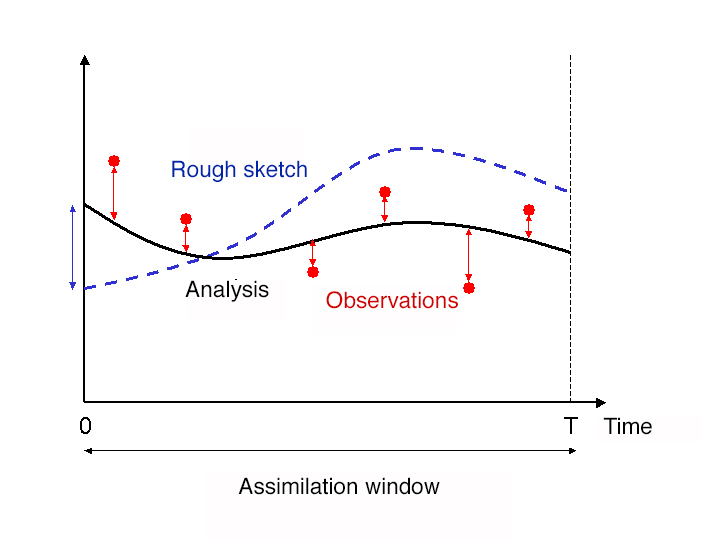
  该方法提出在连续的时间间隔上对观察结果进行分组,并称为同化窗口。对于一个全局模型,这些同化窗口通常持续6小时,并以基本天气观测时为中心(0小时、6小时、12小时、12小时、18小时),在这些时间点上,大气的无线电探空仪会每天运行2-4次。然后,在每个同化窗口的时间起点,我们寻找可以让模型预测起点最接近同化窗口测量值的模型变量集合,它给出了整个同化窗口中最接近测量值的预测起点(因此这个预测是在每个同化窗口的6小时内进行的)。这提供了一种模型变量的状态,该变量来自于在给定的同化窗口期间收集的所有数据,然后可以在几天内据此做出预测。这样可以通过提供同化窗口期间所有收集到的数据来提供模型变量的状态,并可以据此做出几天内的预测。

  这种方法类似于最小二乘法中的最小化问题,其仍然可以用迭代的方法来解决。我们尝试使用四维变分方法(4D-var),4D是因为现在是一个四维问题(3个空间维度,x,y,z,和一个时间维度t)(见图3)。四维变分算法的实现使模型预测能够更好地考虑观测结果,从而提高了预测的质量。

10. 在数据同化方面的预期发展

  增加测量值可以提高预测质量,这种提高在很大程度上是由于数据同化技术的进步。我们目前做了很多工作来更好地说明在预测/修正周期中预测的不确定性。要做到这一点,需要依赖于实现预测/修正周期的两个信息源(预测值和测量值),当然这两者都存在一定的偏差。这种组合预测所提供的预测偏差使我们可以量化预测的不确定性,类似于卡尔曼滤波器,但需要一个恰当的代价函数,即集成卡尔曼滤波器(EnKF)。预测技术的发展方向也存在其他技术路线,例如对与测量相关的不确定性的最佳描述。同化算法类的焦点之一是寻找同化算法公式,这需要借助于未来搭载数百万个处理器的超级计算机上的应用程序来实现!


参考资料及说明

[1] F. Richardson, Weather prediction by numerical process, Cambridge University Press, Cambridge, Reprinted by Dover (1965, New York) with a new introduction by Sydney Chapman, 1922.

[2] Charney, J. G., R. Fjortoft, and J. von Neuman, Numerical integration of the barotropic vorticity equation, Tellus 2, 237-254,1950.

[3] M. Legendre, Nouvelles méthodes pour la détermination des orbites des comètes, Paris, Firmin Didot, 1805.

[4] F. Gauss, Theoria Motus Corporum Coelestium, Ghent University, 1809.

[5] E. Kalman, A New Approach to Linear Filtering and Prediction Problems, Transaction of the ASME – Journal of Basic Engineering, Vol. 82, pp. 35-45, 1960.


The Encyclopedia of the Environment by the Association des Encyclopédies de l'Environnement et de l'Énergie (www.a3e.fr), contractually linked to the University of Grenoble Alpes and Grenoble INP, and sponsored by the French Academy of Sciences.

To cite this article: DESROZIERS Gérald (March 11, 2024), 气象资料同化, Encyclopedia of the Environment, Accessed July 27, 2024 [online ISSN 2555-0950] url : https://www.encyclopedie-environnement.org/zh/air-zh/assimilation-meteorological-data/.

The articles in the Encyclopedia of the Environment are made available under the terms of the Creative Commons BY-NC-SA license, which authorizes reproduction subject to: citing the source, not making commercial use of them, sharing identical initial conditions, reproducing at each reuse or distribution the mention of this Creative Commons BY-NC-SA license.