Weather forecasting models
PDF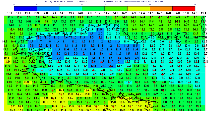
This article presents the basic principles of numerical atmospheric modelling. First, it explains how to move from general and continuous equations of fluid mechanics to a discretized version of these equations. Then it shows how they can be translated into high-performance computer programs, the atmospheric models, which calculate the future state of the atmosphere from an initial state constructed using meteorological observations. The atmospheric model is thus the heart of operational numerical weather prediction systems.
1. What is an atmospheric model?
An atmospheric model is a computer system that simulates the behaviour of the atmosphere. It is used either as a numerical laboratory to study atmospheric processes and better understand them, or as a tool to help predict weather or climate.
The basic laws that describe the evolution of the state of the atmosphere are those of fluid mechanics. They express the evolution over time of a fluid (liquid or gas) from its supposedly known initial state. Their general shape is universal and therefore valid in very different contexts, for example the flow of air around an aircraft, the circulation of water in pipes or rivers, the propagation of sound waves around a wind turbine, or the rise of smoke from a chimney. These equations also make it possible, and this is what we are interested in for atmospheric models, to describe the evolution of the geophysical fluids that are the oceans and the atmosphere.
In the case of the atmosphere, the laws of fluid mechanics are formulated to predict atmospheric parameters such as wind, temperature, pressure and humidity. These are very complex equations because there are many cross interactions between these parameters. These equations also involve processes at very different scales, from the scale of the planet to that of the raindrop, as well as interactions with the underlying surface (land, sea, vegetation cover, see Biosphere, hydrosphere and cryosphere models) and space. Their extreme complexity, due in particular to their non-linearity, precludes their analytical solution. The only way out is therefore to use approximate numerical techniques to calculate the evolution of an initial state. This initial state, called analysis, is itself manufactured using highly sophisticated mathematical and numerical methods for assimilating atmospheric observations (see Assimilation of Meteorological Data).
The atmospheric fluid is essentially a gas composed of dry air (20% oxygen, 80% nitrogen) and water vapour. Other gases such as ozone or carbon dioxide are present with very low concentrations (see The Earth’s Atmosphere and Gas Envelope). However, these minority gases play an essential role in the energy balance of the atmosphere. In the layer where most weather events occur, the troposphere, temperature and pressure conditions can lead to phase changes in the water. Water vapour can thus be transformed into liquid or ice condensates which constitute clouds and precipitation. However, taking into account these phase changes, phenomena with very non-linear thresholds and therefore difficult to translate into equations, is essential to correctly model the behaviour of the atmosphere.
In the context of numerical weather prediction (NWP) (see Introduction to Weather Forecasting), the atmospheric model is one of the links in the “data assimilation – calculation – forecasting” cycle implemented in operational forecast centres. It must not only produce good quality forecasts, but also be fast and robust in order to produce the information needed by forecasters on time and without fail.
2. The equations of fluid mechanics
The Euler system of equations, which expresses the fundamental principles of fluid mechanics and thermodynamics, forms the basis of an atmospheric model. These equations do not apply to a gas molecule but to a parcel of air. It is assumed to be both large enough to contain enough molecules for statistical parameters such as temperature and pressure to be defined and small enough to be assimilated to a point in the vastness of the atmospheric environment.
This system contains three main equations:
- The mechanical equation that expresses the acceleration of the motion of an air parcel as a function of the forces applied to it. In a horizontal plane, this equation gives the wind acceleration as a function of the pressure forces and the Coriolis inertial force due to the Earth’s rotation. On the vertical, the acceleration of the movement is controlled by gravity and by Archimedes’ force.
- The total energy conservation equation which, combined with the equation for kinetic energy deduced from the equation of motion, provides an equation for temperature (or another quantity derived from temperature such as enthalpy or entropy). In particular, it describes the effects on temperature of solar radiation, infrared radiation emitted by the Earth or clouds, and those associated with any change in water status (evaporation cools, condensation heats up).
- The mass conservation equation that ensures the conservation of the different components of an air parcel.
To these three equations, we add the gas state equation which links the three thermodynamic parameters, temperature, pressure and density as well as the thermodynamic laws describing the phase changes of water.
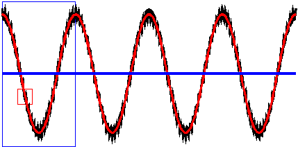
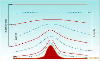
Euler’s equations are able, for example, to describe each small vortex in the vicinity of the Earth’s surface or each diversion of air currents around an obstacle. But the capacity of the computers that will allow us to solve these equations is not yet sufficient to calculate, in practice, the evolution of all these small details. It is therefore necessary to simplify Euler’s equations in order to keep only the essential terms for meteorology. The first step in simplification is to average the original equations in time and space in order to filter the fast and small-scale spatial processes that cannot be described. As a result of this averaging operation, atmospheric parameters such as wind or temperature that are predicted by the equations no longer represent the wind or temperature of a small parcel of air but the average of these parameters in a volume large enough to contain a large number of small eddies and small enough that the averaged parameters still contain the variability necessary to describe the weather phenomena that are to be predicted (Figure 1).
In a second step, the order of magnitude of each of the terms of the equations is analyzed in order to eliminate those that become negligible at the scales still described by the average equations. For example, a classic approximation in atmospheric models is the hydrostatic approximation, which neglects vertical acceleration in the vertical equation of motion. The remaining terms in the equation – gravity and Archimedes’ force – must then balance each other. Consequently, the mean parameters described by the hydrostatic equations (also known as primitive equations) are, by construction, always in hydrostatic equilibrium. In other words, in such a model, the adjustment to hydrostatic equilibrium is treated as a very fast process that is – filtered by the spatial and temporal means applied applied to the equation – then no longer explicitly described by these equations. Hydrostatic equations in particular no longer represent the vertical propagation of acoustic waves, which are so fast that they have little direct interest in meteorology. Their filtering is also an advantage for the stability of numerical models (see section 3). The hydrostatic approximation is valid as long as the atmospheric parameters are averaged in volumes with a horizontal section greater than a few kilometres. However, for finer representations, it may become important to explicitly describe non-hydrostatic transient processes.
The filtering operation, if it removes the possibility of solving every small detail of the atmospheric fluid by the equations, leaves the possibility of representing the collective influence that these fluctuations have on the mean fields. This possibility is particularly important to take into account exchanges with underlying land surfaces (link to article Biosphere, hydrosphere and cryosphere models), which involve very fine and rapid turbulent scale processes. Statistical regression laws that have been established and validated by experience make it possible to link the collective effect of small eddies and micro-circulations in the first few hundred metres above the surface to the average evolution of wind, temperature and humidity in this layer. These statistical laws are the basis for small models, integrated into the global model, called physical parameterizations.
The phase changes of water vapour into droplets or ice crystals that can then evaporate or melt cannot be explicitly described by the averaged equations. To represent them, again, it is necessary to adopt another family of parameterizations based on statistical descriptions of the behaviour of populations of drops or crystals called cloud microphysics schemes.
The modeler has an additional difficulty to represent clouds that are too small to be created by ascents due to the average vertical velocity. Specialized parameterizations to describe clouds of low horizontal extension such as cumulus or cumulonimbus address both vertical velocity fluctuations and water phase changes. These parameterizations, known as convection schemes, are one of the key elements to correctly represent energy exchanges in tropical regions and thus ensure that climate balances are maintained in the model.
It is also necessary to set up all the interactions between the atmosphere on the one hand and, on the other hand, the solar radiation coming from space and the infrared radiation which is mainly emitted by the earth’s surface. These effects must be greatly simplified to make the parameterization of radiation compatible with the constraints of forecast production in the operational centres.
In general, atmospheric system modellers separate the terms of the equations that are expressed directly as a function of the average parameters in a subsystem, called dynamics, from the terms that require the development of parameterizations placed in a second subsystem called physics. It is the coupling between these two subsystems that constitutes an atmosphere model.
3. Discretization and digital algorithms
The equations are not solved independently for each mesh. Indeed, the expression of horizontal and vertical variations of the various quantities as well as that of the transport of these quantities by the wind, involve values in the neighbouring meshes. Parametrizations, on the other hand, often involve calculations along all the meshes of a vertical column (to describe, for example, the rainfall or the turbulent upward transport of water vapour that evaporates at the ocean surface).
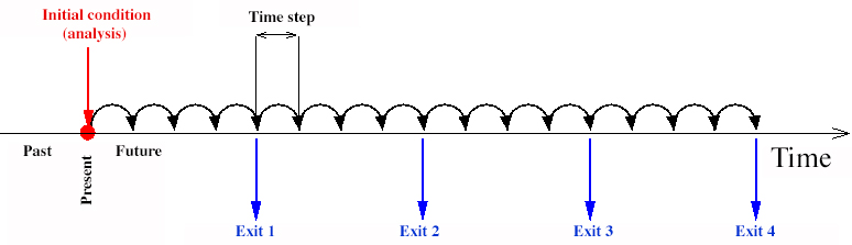
The discretization of the equations does not only occur in space but also in time. The time step, which is the time equivalent of the mesh size in space, separates two successive estimates of the state of the atmosphere by the model (Figure 3).
Numerical schemes, even the most sophisticated ones, are methods of approximate resolution whose solution converges on the exact solution when the patio-temporal resolution of the model becomes very fine. For this reason, the resolution of the models increases as the capacity of the computers increases.
It must be ensured that the error level remains stable during the simulation. Some numerical schemes can indeed see their error grow very quickly if certain conditions are not met. A classical stability constraint, known as the Current-Friedrich-Levy condition or CFL condition [1], specifies that the wind in a mesh must not carry the air present in that mesh more than the size of a mesh in a single step of time. If this condition is not verified in the scheme, the error increases until it reaches infinitely large numbers, the scheme becomes unstable, it is said that the model explodes.
Many modeling schemes have been proposed in the past and new ones are still published every year. The difficulty for the modeler is to make the choices that allow the best compromise between precision, stability and efficiency in computation time. These choices are not independent of the architecture of the computer that will be used.
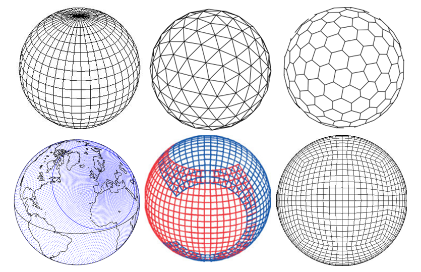
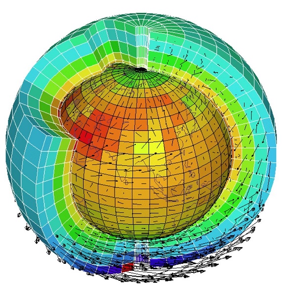
Even if all models are based on the same system of equations, in practice, each implementation can vary widely from one model to another. On the horizontal, there is a wide variety of possible mesh sizes (Figure 4) ranging from a simple regular grid along circles of latitude and meridians to grids with hexagonal or triangular meshes. Some stranger meshes, such as the cube sphere or the Yin-Yang grid, have interesting mathematical properties, in particular, they do not present any singularity at the poles. In some cases, the type of grid is imposed by the chosen numerical method. The global model of Météo-France and the model of the European Centre for Medium-Range Meteorological Forecasting (ECMWF) use a mathematical transformation that projects the parameter fields on the basis of mathematical functions, the spherical harmonics. For this transformation to be accurate, it is necessary to use a Gaussian grid [2]. In Météo-France, the grid is also stretched to increase the resolution over France.
In addition to global models that produce forecasts for the entire atmosphere and that also often have a version used for long-term forecasts, such as seasonal or climate forecasts, there are many regional models that computation only for a given region. The reduction in the number of calculation points in these limited area models allow an increase in resolution and a better optimization of the tuning for this region. One of the limitations of regional models is the need to couple the solution on the edges of the limited domain with the solution provided by a lower global resolution model. Coupling techniques are important sources of errors that spread within the area of interest and thus limit the duration of this type of forecast.

The fields provided by the model are not stored at each time step but only for the forecast times required by the users. The raw parameter fields such as temperature, wind or geopotential height are interpolated to the isobaric levels conventionally used by forecasters. Cloud cover and surface precipitation are provided directly by the cloud parameterizations. Many other parameters are diagnosed from the model’s raw outputs to help the forecaster analyze the behaviour of the atmosphere and compare the predicted states with new observations that arrive in real time. Maps of surface parameters such as temperature at 2 m above the surface, wind at 10 m above the surface, gusts, but also satellite images or synthetic radar images (Figure 6) are thus routinely processed. Model outputs are the main information that is made available to expert forecasters (see The Role of the Forecaster). They use it to produce the best general scenario for the weather evolution in the coming days and the necessary refinements for each region around the globe.
4. The challenge of computer programs and supercomputers
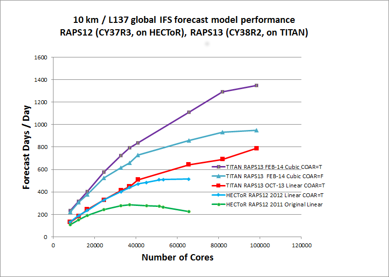
The forecasting models which are operational in 2016 include several million meshes, about ten variables per mesh and time steps of a few minutes. They require the solution of more than 100 million complex equations to produce a single hour of forecast. Only the use of the most powerful computers, but also efficient algorithms, can produce forecasts quickly enough to be transmitted to forecasters in a time.
An atmospheric model is therefore finally a computer code of several million lines, developed and maintained by dozens of people in parallel. It is the heart of the data assimilation and high-resolution forecasting cycle in operational weather forecast centres. It is also used to produce the perturbed forecasts of each member of the ensemble forecast (see The ensemble forecastting). Coupled with an ocean model, it is used for monthly and seasonal forecasts and to monitor climate change (see The Seasonal Forecast).
Numerical modelling of the atmosphere has had to and must continue to cope with:
- increases in resolution and therefore in the number of calculations,
- increases in the processes to be described (e.g., addition of atmospheric chemistry),
- increases in the number of processors in the ECUs,
- increases in power consumption of supercomputers,
- increases in the number of program lines,
- increases in the mass of data to be processed and stored at the output.
An important challenge in the coming years is to improve the scalability of existing models, i.e. their ability to adapt to all these increases, while remaining tools that can still be used by all researcher-developers and are still useful for weather forecasting applications.
References and notes
Cover image: Forecast of temperatures over Brittany on 10 October 2016 for 17 October 2016 at 00 GMT using the ECMWF digital model (black figures: temperatures in °C; red crosses: mesh centres).
[1] J. Coiffier : Éléments de prévision numérique du temps, “Cours et Manuel”, 1997, Météo-France.
[2] S. Malardel, N. Wedi, W. Deconinck, M. Diamantakis, C. Kuhnlein, G. Mozdzynski, M. Hamrud, P. Smolarkiewicz : A new grid for the IFS, 2016, ECMWF Newsletter 146.
[3] S. Malardel : Fundamentals of Meteorology, 2nd ed., 2009, Cépadues éditions.
The Encyclopedia of the Environment by the Association des Encyclopédies de l'Environnement et de l'Énergie (www.a3e.fr), contractually linked to the University of Grenoble Alpes and Grenoble INP, and sponsored by the French Academy of Sciences.
To cite this article: MALARDEL Sylvie (January 5, 2025), Weather forecasting models, Encyclopedia of the Environment, Accessed July 13, 2026 [online ISSN 2555-0950] url : https://www.encyclopedie-environnement.org/en/air-en/weather-forecasting-models-2/.
The articles in the Encyclopedia of the Environment are made available under the terms of the Creative Commons BY-NC-SA license, which authorizes reproduction subject to: citing the source, not making commercial use of them, sharing identical initial conditions, reproducing at each reuse or distribution the mention of this Creative Commons BY-NC-SA license.