The tides

PDF

Tide refers to the process of periodic sea level change, usually semi-diurnal (period close to 12 hours), but diurnal in some regions. The tide is due to the lunar attraction, and to a lesser extent to the attraction of the Sun which modulates its amplitude according to the phase of the Moon and different astronomical periods. Very violent local currents are associated with tides in coastal areas. In addition to these well-known local effects, the tide plays a global role in climate by contributing to the vertical mixing of the ocean. Tidal oscillation excites internal waves propagating along interfaces due to temperature differences within the ocean, producing mixing as they break. Finally, on a geological time scale, the tide slows down the Earth’s rotation and keeps the Moon away from the Earth.

1. Observations from antiquity

The links between the tide and the movement of the Moon have been known empirically from antiquity [1]. The time of low water (minimum level) and high water (maximum level)  delays by about 25 minutes per tide, or 1/60th day, corresponding to the displacement of the Moon on its orbit by 1/60th of a turn in 12 hours (1 turn in 30 days). Because of this delay the effective tidal period is 12 h 25 mn. It is also known that tides are more intense during the full and new Moon (spring tides) than during the first and last districts (neap tides). This indicates that the effect is governed by the Moon, with a more modest contribution from the Sun. The tide is particularly strong at equinoxes and also depends on the distance from the Moon, which varies by about 10% because of its elliptical orbit. The tidal amplitude in a given place is thus modulated by a tidal coefficient that can vary from 20 to 120 according to the different astronomical periods.

height water tides
Figure 1. Record of sea level at different sites. [Source : © Shom – Extrait du guide “La marée”]
Tidal range, the difference in height between low water and high water, also depends greatly on the location, with the highest values reaching nearly 18 m in Ungava Bay (Quebec), 16.5 m in the Severn Estuary (Great Britain) and 15 m at Mont Saint-Michel (France). However, it is limited to a few tens of centimetres in other parts of the ocean. Moreover, this predominantly semi-diurnal oscillation, typical of the Atlantic coasts, is not observed everywhere, as the curves in Figure 1 show [2]. We will come back to this later.

Due to its elasticity, the solid Earth is also subject to a tidal effect but with a smaller amplitude, in the order of 10 cm. What we observe at the seaside is the difference between the ocean tide and this land tide. Older measurements were made near the shore by float gauges, more recently replaced by ultrasonic or radar water level detectors. Altimetry satellites now allow tide mapping over the entire oceanic surface by radar measurement, after calibration by buoys whose position is tracked by GPS.

2. Newton’s static theory

Tides were very early interpreted as an attraction effect of the Moon and the Sun. However, these explanations stumbled on the fact that the sea is raised not only on the side of the Moon, but also on the opposite side, leading to the 12-hour period (rather than 24 hours). It was Isaac Newton (1643-1727) who first understood this paradox thanks to his theory of universal gravitation published in 1687 in his famous book Philosophiae Naturalis Principia [3]. Tides play an important role because they were the most tangible effect of attraction by a body outside the Earth at that time.

schema theory static Newton
Figure 2. a) Scketch of the ‘static theory’ of Newton; b) More realistic sketch taking into account the entrainment of water by Earth’s rotation, leading to a shift of the bulges. This shift induces a torque which progressively slows down Earth’s rotation and drives away the Moon (see section 8).

Newton first understood that if the Earth keeps the Moon in orbit by its attraction force, the Moon must in turn exert an equal and opposite force on the Earth: this is the principle of action and reaction. Thus the Earth revolves a little around the Moon, more precisely around their common barycentre (point G in Figure 2). Every body on Earth accompanies it in its movement around this barycentre, in the same way that an orbiting cosmonaut remains weightless near his spacecraft. The reason is that every body undergoes the same acceleration in a field of gravity regardless of its mass. What will move the ocean relative to the Earth is therefore not the attraction field of the Moon, but the difference between this field and the one acting at the centre of the Earth. An excess attraction is exerted in the areas closest to the Moon and a lack of attraction on the opposite side further away, producing a bulge on each side, as shown in Figure 2. Another equivalent argument is to place oneself in a frame of reference rotating around this barycentre at the orbital angular velocity of the Moon: the centrifugal force then compensates for the lunar attraction at the centre of the Earth, but it dominates at the point opposite the Moon, while the attraction dominates on the Moon’s side. This leads to the two bulges respectively.

In the so-called static theory proposed by Newton, these bulges are assumed to be fixed in relation to the Earth-Moon system. During its rotation around the Earth, a point thus passes successively through each bulge leading to two high tides per day, hence the semi-diurnal period.

The effect of the Sun is added to that of the Moon when it is in the same direction (new Moon), but also when it is in the opposite direction (full Moon), due to the double bulge. This explains the alternation observed between spring tides and neap tides. The attraction force of the Sun is stronger than that of the Moon, but the difference between the two sides is smaller due to the long distance, producing a lower tidal effect . Thus the gravitational attraction decreases as the square of the distance while the corresponding tidal effect decreases as the cube of the distance.

3. Tidal amplitude variations

A complication comes up from the fact that these different rotations occur along different axes: the Earth’s axis of rotation is tilted by 23°26′ with respect to the plane of the Earth’s orbit, itself close to the plane of the Moon’s orbit (inclined by 5° 9′ with respect to the plane of the Earth’s orbit). The diagram of  Figure 2 applies strictly to the equinoxes, when the axis of rotation is  transverse to the direction of the Sun, aligned with the Moon at spring tide.

However, at the solstices, a point on the Earth travels around the bulges in an inclined circle, leading to a smaller amplitude. This can be understood by considering the limiting case of a 90° tilt: at the solstice the Earth’s axis would then be oriented along the axis of the bulge, and a point on Earth would then rotate around it without any variation in height, like a rugby ball rotating around its major axis.

Finally, the Moon’s orbit is not circular, but elliptical, so that the distance D to the Earth varies by 10% between the perihelion (minimum) and the aphelion (maximum). As a result, the tidal effect is greater at perihelion by 30% (due to the dependence in 1 / D3). These different astronomical effects are taken into account in a very precise way to establish the tide tables. The understanding and prediction of tides has been the subject of much work throughout the 19th and 20th centuries (focus 1) because of its fundamental interest and importance for navigation and coastal use.

4. Tidal waves

Newton’s static approach assumes that the ocean bulge, which is fixed relative to the Moon, propagates relative to the Earth at the speed opposite to its rotation, i.e. 450 m/s at the equator. This is not possible because a deformation of the ocean surface propagates at a limited speed of about 200 m/s. This speed is related to the ocean depth d and the acceleration of gravity g by the formula c=(gd)1/2 (read https://www.encyclopedie-environnement.org/eau/vagues-houles/). This yields c=200 m/s for an average depth of d=4000 m. This wave therefore lags behind the position of the Moon, which leads to a shift of the bulge as shown in Figure 2b.

The shape of the coasts also strongly constrains this propagation, with ocean basins behaving like large basins of water shaken by the tidal force. There are established specific modes of oscillation, somewhat similar to the modes of vibration of sound waves in a musical instrument.

amplitude phase tide
Figure 3. Amplitude and tidal phase M2 (semi-diurnal period) measured by the altimetric satellite Topex-Poseidon. The colours represent the amplitude (the tidal range is twice the amplitude), and the white lines the phase, i.e. the time separating the maximum from the passage of the Moon to the zenith.

Newton’s theory remains accurate as a driving force, but the resulting deformation therefore depends on these propagation phenomena and the resonances that occur when the excitation frequency coincides with the natural oscillation frequencies of ocean basins.

Tidal amplitude is now mapped with centimetre accuracy using altimetry satellites (see Figure 3). We can see that the amplitude is very variable, with oscillation antinodes (maxima in red) and oscillation nodes where the amplitude cancels (in blue). The lines of equal phase are also shown: they represent the delay of the tidal maximum with respect to the passage of the Moon at zenith. The tidal wave propagates perpendicular to these lines, thus rotating around the nodes. This rotation, due to the Coriolis force, is counter-clockwise in the Northern Hemisphere.

The modulation of the tides by the different astronomical effects is more precisely expressed as a sum of excitations at different periods, the semi-diurnal mode being however dominant. It is this mode, called M2, which is represented in Figure 3. Note that the average distance between antinodes (or between nodes) corresponds to the tidal wavelength of the order of 8500 km, i.e. the distance travelled by the wave at speed c=200 m/s during the 12 h period.

There is also an excitation at the diurnal period, resulting from a slight asymmetry of the two opposing bulges of attraction. This mode, called M1, is forced to a level 20 times weaker than M2, but it effectively resonates with the Pacific Ocean, which is comparable in size to its wavelength, about 15,000 km. The diurnal tide is thus significant in some regions of the Pacific. Regions located on nodes of the M2 mode, such as Vietnam, then mainly feel this M1 mode (3rd curve in Figure 1). Other regions show a superposition of both M1 and M2 modes (2nd and 4th curves in Figure 1).

model handle coriolis
Figure 4. Physical scale model of the English Channel on the large “Coriolis” rotating platform at Grenoble, France.

The tidal wave is often amplified in bays or inland seas such as the English Channel. This is because the energy propagates more slowly, as a square root of the depth, resulting in an increase in energy density at constant flux: moving from 5000 m to 50 m thus produces an increase in energy density by a factor of 10, i.e. an increase in amplitude by a factor of 3. In the English Channel, the average amplitude typically increases from 1 m offshore to 3 m, and the tide is associated with a strong current. The incoming current is deflected towards the French coast by the Coriolis force, and away from it at ebb tide, which amplifies the tidal range on the French side, to the detriment of the English side. These effects could be reproduced in a similar way on the large “Coriolis” rotating platform, shown in figure 4. The ocean tide forcing is then reproduced by an oscillating beater located at the entrance to the English Channel. The amplitude and phase of the tide over the whole of the English Channel could thus be reproduced (Figure 5).

iso amplitude iso phase coriolis
Figure 5. Iso-amplitude (top) and Iso-phase (bottom) curves measured on the Coriolis platform. The experimental curves (dotted lines) are compared with the observations (solid lines). It can be seen that the amplitude is particularly strong in the Bay of Mont Saint-Michel, while the phase lines characterise the propagation of the tidal wave in the Channel

Current numerical models make it possible to reproduce and predict these tidal phenomena with an accuracy of around 1cm. The main difficulties are the consideration of friction on the ocean floor in turbulent conditions and energy losses due to internal tidal excitation (see section 7).

5. Other influences on sea level

The tide is not the only effect influencing sea level. First of all, we can ask ourselves about the relevance of measurements to the nearest cm in a sea that is often rough with waves of several metres. But the average level over several square kilometres is very well defined even if it locally fluctuates very strongly. In addition, for tidal amplitudes such as those in Figure 3, the signal is filtered at a given time period (12h 25 min), similar to the frequency selection used to receive radio waves. Thus, effects acting at other frequencies are not taken into account.

Among these other effects, atmospheric pressure is a fairly immediate factor. A high pressure locally lowers the water level: an overpressure of 10 hPa = 103 N/m2 induces by simple hydrostatic equilibrium a decrease of the level by 10 cm, the height h of a water column whose weight ρgh is 103 N/m2 (ρ=103 kg/m3 represents the density of water). By contrast low atmospheric pressure raises the water level. The overheight reaches a value of one metre at an atmospheric pressure of 913 hPa, occurring in the middle of extreme hurricanes. This rise in water levels amplifies the damage caused by waves and heavy rainfall in coastal areas.

A second effect  is due to the friction force of the wind. When it is directed offshore, this force lowers the water level, and by contrast pushes the water towards the shore if it is directed toward the land. An elevation of about 1 m can be produced during heavy storms. The coincidence of these phenomena with high tides favours the breaking of protective dikes that cause flooding, such as the storm “Xynthia” that struck France in February 2010, or hurricane “Katrina” that flooded New Orleans in August 2005. These phenomena, depending on wind and pressure, are however much more predictable than the intense and very local precipitation that causes flash floods.

In the longer term, average sea level increases in the presence of global warming due to ocean expansion, which accounts for about 65%, and glacier melting for the remaining 35%. Recent measurements indicate an average elevation of about 2 mm/year.

Finally, the water level on the coast also depends on the evolution of the solid Earth. Sediment transport modifies the shoreline, through siltation or erosion. The latter effect currently tends to dominate due to dams on large rivers that reduce sediment input. The Louisiana coast is severely eroded due to the decrease in sediment brought by the Mississippi River. Deep geological movements also contribute, changing the shape of the coasts by continental drift over millions of years. In Canada and northern Europe, the most significant geological effect is the post-glacial rebound that raises Scandinavia by several mm per year following the load reduction due to the melting of the ice caps 10,000 years ago. This uplift induces by compensation a sinking of peripheral areas such as Brittany in France. Thus, menhirs erected on land 7000 years ago are found in the sea, after a sinking of the continent by about 7 m.

6. Harnessing the energy of the tide

Tidal mills have been used since the Middle Ages to harness tidal energy at favourable sites, with estuaries or coves sheltered from the waves and equipped with small dams. The principle was adopted for the Rance tidal power plant, which was commissioned in 1967. With an average capacity of 57 MW (installed capacity of 240 MW), it produces 3.5% of Brittany’s electricity consumption (and 45% of its electricity production). It remained the world’s largest tidal power plant for 45 years, until the slightly more powerful Sihwa Lake power plant in South Korea was commissioned in 2011 (254 MW installed). The facility uses a dam across the Rance estuary, with directional blade turbines that can operate in both directions, at rising or falling tide.

However, few high tide sites allow the construction of facilities of this size, and the need to preserve natural sites now makes it difficult to build them by the sea. A much more ambitious project consisted in damming the bay of Mont Saint-Michel in France. This is a particularly exceptional site in terms of tidal amplitude, but this project was abandoned in favour of the development of nuclear power plants in the 1970s.

amplitudes velocities tidal currents
Figure 6. Map of the velocity amplitudes of tidal currents, and prototype installation sites on the Breton coast: Raz de Sein, Ouessant and Raz Blanchard. In insert, turbine model developed by the company Electricité de France (diameter 10 m).

The current trend is to directly use the currents produced by the tide through hydro turbines, the marine equivalent of wind turbines. These turbines do not require reservoirs and therefore have a lower environmental impact. However, the developments are only at the prototype stage of a few MW, with test sites in Scotland and Brittany (see Figure 6). In Scotland, the objective by 2020 is to build hydroelectric farms producing 1,000 MW. The total estimated resource in Europe is around 10,000 MW installed (5,000 MW average), 80% of which is in France and Great Britain. This represents about 10% of the average electrical power consumed in France.

This resource represents barely 0.2% of the total power dissipated by the tides and thus lost through the Earth’s rotation (see section 8). Energy extraction tends to slow down the tidal current and thus reduce its amplitude locally, thus reducing viscous friction losses. It can be expected that the extracted energy will be dissipated as heat anyway in the absence of capture. However, it is not easy to calculate the return impact on the Earth’s rotation, which is very small anyway[5].

7. Internal tide

The density of the ocean increases with depth, with surface water being warmer (and therefore less dense) than deep water. Such density stratification can also result from salinity, for example in the Strait of Gibraltar where ocean water enters the more salty Mediterranean Sea while remaining at the surface due to its lower density. This situation can be summarized by a two-layer model of different densities.

Internal wave oscillations, known as internal waves, can propagate along this interface in a similar way to surface waves. However, they are much slower, described by replacing gravity g by a reduced gravity gδρ/ρ, where δρ/ρ is the relative density difference between the two layers. In a surface layer of thickness H, the propagation velocity of the waves is therefore c=(Hgδρ/ρ)1/2 . For or a typical value δρ/ρ=0,001, the propagation speed is thus 30 times less than for the surface waves in a layer of the same thickness : c=1 m/s for a layer of thickness H=100 m.

tide impact roughness oceanic surface
Figure 7. Internal tide visualized by its impact on the roughness of the ocean surface. Sulu Sea between the Philippines and Borneo. The distance between two wave trains, produced 12 hours apart, is about 100 km. [Source : satellite photo https://earthobservatory.nasa.gov/images/3586/internal-waves-sulu-sea]
The tide carries a horizontal current over the entire water level. However, as a slope passes, this current acquires a vertical component that deforms the interface and thus generates an internal wave, called in this case the internal tide. These waves have a wavelength of about 100 km (distance travelled at 1 m /s during the 12-hour tidal period). In addition, they tend to be located in solitons, compact waves of high amplitude (Figure 7). Although these waves propagate at depth, the horizontal currents they generate are seen on the surface by changing wave shapes that change the brightness of the sea.

Internal tidal generation is observed in many parts of the ocean. One of the most active is the Strait of Luzon, separating Taiwan and the Philippines, where an underwater ridge generates internal waves in the China Sea whose vertical displacement exceeds 300 m. The dissipation of these waves by breaking contributes to the vertical mixing of the ocean, which in turn affects its general circulation and climate.

8. Astronomical effects and energy dissipation

On astronomical time scales, the tides increase the length of the day by 2 ms per century, or about one hour in 200 millions years. This slowing down of the Earth’s rotation can be measured very well with current atomic clocks. In addition, the tidal effect moves the Moon away by 3.8 cm/year. This effect can be measured directly with an accuracy of 1 cm by measuring the round trip time of laser pulses sent to reflectors deposited by the Apollo lunar missions [7].

This slowdown is confirmed by the observation of fossil corals (ref 6), whose daily growth circles make it possible to count the days in a year. Thus the year counted 410 days 400 million years ago, a 21.5-hour day. Monthly bands associated with the full moon also indicate that the year was 13 months long, i.e. the Moon was spinning faster (and was therefore closer to the Earth).

These effects are easily understood with the diagram in Figure 2b. Earth’s rotation tends to entrain the bulge, which is therefore out of phase with Newton’s static model. The lunar attraction thus exerts a torque that slows down the Earth and reciprocally brings energy to the Moon. Counterintuitively at first sight, such an energy supply tends to drive away the Moon, and therefore to slow down its rotation, whose speed decreases in 1/√r. However, the kinetic moment of the Moon, produced by the speed by the distance to the Earth r increases well (in √r), in accordance with the motor direction of the torque. The kinetic moment of the Earth decreases in the same proportion so that the total kinetic moment is preserved. The total mechanical energy decreases, converted into heat when the marine currents produced by the tide dissipate.

Astronomical measurements make it possible to accurately determine the decrease in rotational energy and thus to deduce the total power dissipated by the tides: 2.9 x10¹² Watts. Oceanographers, for their part, have estimated a power dissipated by about half by studying tidal currents, most of which are active in coastal areas. It is now established that the’missing dissipation‘ is due to the excitation of the internal tide (see section 7), which spreads inside the ocean and eventually dissipates. This dissipation occurs by waves breaking, producing a slow vertical mixing of the ocean. The influence of these effects on thermo-haline circulation is currently under active research.


Notes and references

Cover illustration. Mont-Saint Michel, où les marées peuvent atteindre un marnage de 15m. source https://upload.wikimedia.org/wikipedia/commons/thumb/2/29/Mont-Saint-Michel_Drone.jpg/1280px-Mont-Saint-Michel_Drone.jpg .

[1] http://www.imcce.fr/promenade/pages5/525.html#Para02

[2] Tidal level records at more than 900 sites over the world are available on http://www.ioc-sealevelmonitoring.org/

[3] Newton I. (1687) ’Philosophiae naturalis principia mathematica’

[4] http://science.nasa.gov/media/medialibrary/2000/06/15/ast15jun_2_resources/oceantides.gif

[5] Maitre T., http://encyclopedie-energie.org/notices/les-hydroliennes

[6] This statement needs to be qualified, as a large energy extraction would in turn change the shape and phase of the tides, and thus the torque exerted on the Earth. nevertheless, a 5,000 MW extraction represents just 0.2% of the total power dissipated in the tides (see section 8)

[7] http://culturesciencesphysique.ens-lyon.fr/ressource/laser-distance-terre-lune.xml

[8] Runcorn S.K. , « Corals as paleontological clocks», Scientific American, vol. 215,‎ 1966, p. 26–33


The Encyclopedia of the Environment by the Association des Encyclopédies de l'Environnement et de l'Énergie (www.a3e.fr), contractually linked to the University of Grenoble Alpes and Grenoble INP, and sponsored by the French Academy of Sciences.

To cite this article: SOMMERIA Joël (October 19, 2021), The tides, Encyclopedia of the Environment, Accessed July 27, 2024 [online ISSN 2555-0950] url : https://www.encyclopedie-environnement.org/en/water/the-tides/.

The articles in the Encyclopedia of the Environment are made available under the terms of the Creative Commons BY-NC-SA license, which authorizes reproduction subject to: citing the source, not making commercial use of them, sharing identical initial conditions, reproducing at each reuse or distribution the mention of this Creative Commons BY-NC-SA license.

潮汐

PDF

  潮汐是指海平面周期性变化的过程,周期通常是半天(接近12小时),但在某些地区是一天。潮汐由月球引力引起,在一定程度上也受太阳吸引,潮汐幅度会随月相和不同的天文周期而变化。沿海局地猛烈的洋流也与潮汐有关。除了这些众所周知的局地作用之外,潮汐通过促进海水的垂直混合而影响全球气候。潮汐振荡所激发的内波沿海水温差界面传播,并在波浪破裂时促使海水混合。最后,在地质时间尺度上,潮汐减慢了地球自转的速度,并使月球远离地球。

1. 自古以来的观察

  古人们已经通过经验了解到潮汐与月球运动之间的联系[1]。每次潮汐中低潮(低水位)和高潮(高水位)的出现相差约25分钟,即1/60天,与月球12个小时公转1/60周(公转周期约30天)相符合。由于这个时间差,实际的潮汐间隔时长为12 小时 25 分钟。且众所周知的是,与上弦月和下弦月(春潮)期间相比,在满月和新月(露潮)期间的潮汐更猛烈。这表明潮汐主要受制于月球,而受太阳的影响则较小。潮汐在二分日时特别强烈,其强度取决于距月球的距离,由于月球公转轨道是椭圆形的,该距离还存在约10%的波动。地表某特定位置的潮汐振幅由潮汐系数描述,根据天文周期的不同,潮汐系数在20-120范围内变化。

环境百科全书-潮汐-不同地点的水位记录
图1. 不同地点的水位记录(©摘自Shom-Extrait《潮汐》)
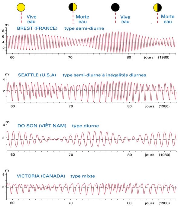
(图中:Vive eau-活水;BREST(FRANCE) 法国布雷斯特;Morte eau-死水;type semi-diturne 半日潮型;SEATTLE 美国西雅图;type semi-diturne à inègalites diurnes 不规则半日潮型;DO SON (Viètnam) 越南涂山;type diurne 全日潮型;VICTORIA(CANADA)加拿大维多利亚; type mixte 混合潮型;jours 天数)

  潮是指高低潮之间的潮位差,很大程度上也取决于地理位置。在加拿大魁北克翁加瓦湾、英国塞文河口和法国诺曼底圣米歇尔山,最高潮差分别达到18米、16.5米和15米,但在其他地区,最高潮差通常为几十厘米。另外,正如图1[2]中的曲线所示,这一显著的半日潮震荡在大西洋海岸比较典型,但并非在每个地方都可以观察到。我们在下文中将回到这一点。

  由于弹性作用,地球的固体部分也存在潮汐效应,但幅度仅为10厘米级别。我们在海边观察到的,即为海洋潮汐与陆地潮汐之间的这种差异。之前的测量是在岸边用浮标测量的,最近用超声波或雷达水位探测器取代。测高卫星现在可以通过雷达测量,在通过GPS跟踪位置的浮标进行校准后,绘制整个海洋表面的潮汐图。

2. 牛顿静力学理论

  潮汐很早就被解释为月球和太阳的引力效应。但是,这种解释与海面不仅在一天中面向月亮时升高,在背对月亮时也升高,且周期是12小时(而不是24小时)的事实相违背。艾萨克·牛顿(1643-1727)在1687年发表的著作《自然哲学的数学原理》中,通过万有引力理论首次解释了这一悖论[3]。潮汐是地表上受地外引力影响最为显而易见的现象,因此具有重要研究价值。

环境百科全书-潮汐-牛顿力学
图2.(a)牛顿静力学理论示意图; b)实际上,由于地球自转引起两侧涨潮强度不同,地月系统出现了一对相互作用力,使地球自转逐渐减慢,并驱离月球(详情见第8节)

  牛顿首先通过作用力反作用力定律表明,如果地球引力使月球沿一定轨道旋转,那么月球一定会对地球施加大小相等、方向相反的力。因此地球也算是绕月球旋转,更精确地说是围绕它们的引力中心(图2上的G点)旋转。地球上的每个部分都与地球一起绕这个中心旋转,就像宇航员在沿轨道飞行的飞船附近会保持无重力状态、与飞船共同飞行一样。其原因就是每个物体在重力场中都会受到与自身质量无关的、大小相同的加速度。因此,使海洋相对于地面运动的原因不在于月球对海洋的引力场,而是该引力场与月球对地球重心的引力场的差值。更靠近月球的一侧引力更大,而距离较远的另一侧则较小,从而在两侧都涨潮(见图2)。另一个等效的论证是将自己置于以月球轨道角速度围绕该重心旋转的参考系中:离心力随后补偿了地球中心的月球引力,但它在月球对面的点上占主导地位,而引力在月球一侧占主导地位。这分别导致了两个凸起。

  根据牛顿静力学理论,假定涨潮位置相对于地-月系统位置固定,则在地球自转时,地面上的某点在一天中能先后经过两个涨潮位置,导致每天有两次高潮,因此潮汐周期为半天

  当太阳和月球同升同落(新月)以及太阳和月球位于对立方向(满月)时,由于两侧海面上升的现象,在月球对潮汐影响的基础上,补充考虑太阳对潮汐的影响。这个补充解释了所观测到的春潮与露潮的交替出现的现象。太阳的引力比月亮大,但由于地日距离更大,太阳在近日侧和远日侧形成的引力场差异较小,因此,引力吸引随距离的平方减小,而相应的潮汐效应随距离的立方减小。

3. 潮汐幅度变化

  由于地球自转、地球公转和月球公转轨道平面不同,导致潮汐更加复杂多变。其中地球自转轴相对于地球公转轨道平面倾角为23°26’,且公转轨道平面接近月球轨道所在平面(相对于地球公转轨道平面倾角为5°9’)。图2的图示严格适用于二分日,当旋转轴横向于太阳的方向,在大潮时与月亮对齐时。

  然而,地球的自转轴在“至暑点”和“至寒点”朝向或背离太阳,而在二分日均匀受太阳直射。我们可以通过假想地球自转轴与公转轨道平面的倾斜角度为90°的极限情况来说明:即地球的自转轴在二至日时会沿着地-日连线指向太阳,那么则有地球上任意一个点的高度将不再随旋转而改变的结论。另一方面,在二分日时,自转轴会与两侧涨潮位置的连线垂直,则地球上的某点点将围绕它旋转,而高度没有任何变化,就像橄榄球围绕其主轴旋转一样。地球上的某点将能连续通过潮涨和潮落为位置。因此活水的潮汐在二分日强于二至日就可以理解了。

  最后,由于月球的轨道不是圆形,而是椭圆形,月球到地球的距离D在近地点(最小)和远地点(最大)相差约10%,因此近地点的潮汐效应比远地点强30%(与1/D3成正比)。在建立潮汐表时,需要非常精确地考虑这些不同的天文效应。在整个19世纪和20世纪,对潮汐的理解和预测一直是许多工作的主题(重点1),因为它对航行和沿海使用具有根本的兴趣和重要性。

4. 潮汐波

  牛顿静力学理论假设海洋的两侧涨潮位置相对于月球固定,因此潮汐能够以地球自转反向速度传播,赤道处的速度将达到450 米/秒。但由于海洋表面的形变,这种传播速度被限制在约200 米/秒以内(图2b)。该速度通过公式c=(gd)1/2与海洋深度d和重力加速度g相关(https://www.encyclopedie-environnement.org/eau/vagues-houles/)。这就产生了c=200 米/秒,平均深度为d=4000米。因此,这种波滞后于月球的位置,这导致了凸起的移动,如图2b所示。

  此外,海岸的形状也极大地限制了潮汐传播,海洋盆地就像潮汐冲刷形成的水池一样。已经发现的一些潮汐的波动形式,有点类似于乐器中声波的振动。

环境百科全书-潮汐-高空卫星
图3. 高空卫星Topex-Poseidon测得的振幅和潮汐相位M2(半日周期)。颜色代表振幅(潮差是振幅的两倍),白线表示相位,即月球到达天顶时与潮汐达到最大值的相差时间。

  牛顿力学作为潮汐驱动力的原理仍然是准确的,但潮汐的具体结果取决于上述传播现象以及潮汐的激发频率与海洋盆地的自然振荡频率一致时的共振现象。

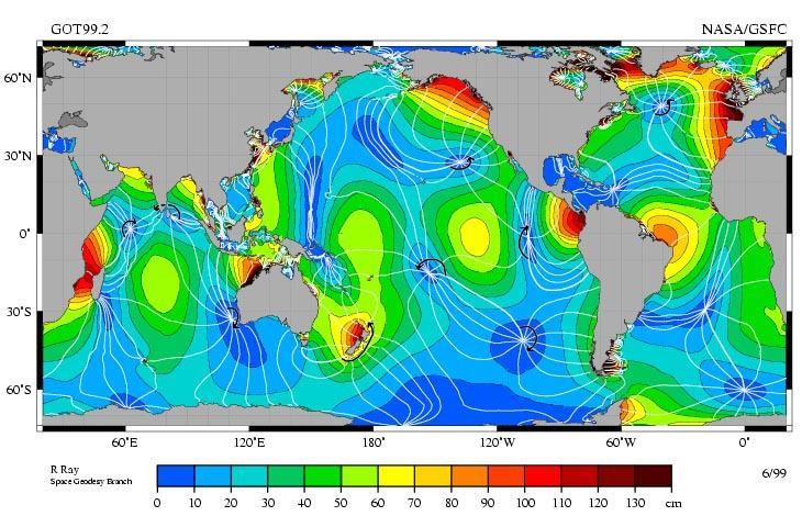
  目前,使用高空卫星可以将潮汐振幅的测量误差控制在一厘米以内(如图3)。我们从图上可以看到振幅大小的多变性,红色表示振荡的峰值,蓝色表示振幅为零的振荡节点。图上的等潮差线表示潮汐峰值与月球到达天顶时的延迟。潮汐波垂直于这些线传播,即围绕某个节点旋转。由于地转偏向力,这样的旋转在北半球是逆时针方向。

  不同天文效应对潮汐的调制更准确地表示为不同时期的激励之和,然而半日模式占主导地位。这就是这种模式,称为M2,如图3所示。注意波腹之间(或节点之间)的平均距离对应于8500公里量级的潮汐波长,即波浪在12小时期间以速度c=200米/秒行进的距离。

  在昼夜周期也有一种应激反应,这是由于两个相对的吸引力凸起的轻微不对称造成的。这种被称为M1的模式被迫达到比M2弱20倍的水平,但它实际上与太平洋产生了共鸣,太平洋的大小与其波长相当,约为15000公里。因此,在太平洋的一些地区,昼夜潮汐非常显著。位于M2模式节点上的地区,如越南,则主要感受到这种M1模式(图1中的第三条曲线)。另外,区域显示了M1和M2模式的叠加(图1中的第2条和第4条曲线)。

环境百科全书-潮汐-高空卫星
图4. 在大型旋转平台《科里奥利》上的英吉利海峡模型。法国格勒诺布尔

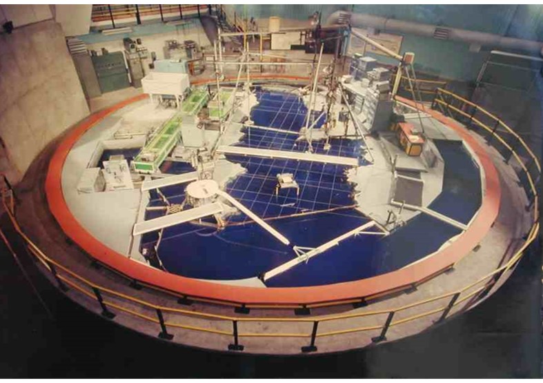
  潮汐波经常在海湾或内陆海(如英吉利海峡)被放大。这是因为能量传播得更多缓慢地,与深度的平方根成正比,导致在恒定通量下能量密度的增加:从5000米移动到50米从而使能量密度增加10倍,即振幅增加3倍。在英吉利海峡,平均振幅通常从离岸1米增加到3米,潮汐与强流有关。流入的水流在地转偏向力的作用下转向法国海岸,并在退潮时离开,这会放大法国一侧的潮差,对英国一侧不利。这些效果可以在位于英吉利海峡的入口的大型“科里奥利”旋转平台(如图4所示)。因此,整个英吉利海峡的潮汐幅度和相位可以被复制(图5).

环境百科全书-潮汐-振幅和相位曲线
图5. 在科里奥利平台上测得潮汐在实验时的振幅和相位曲线。用虚线在图上表示,并与观测得到的图上实线比较。可以看到圣米歇尔山的振幅非常大,英吉利海峡潮汐的相位变化明显。

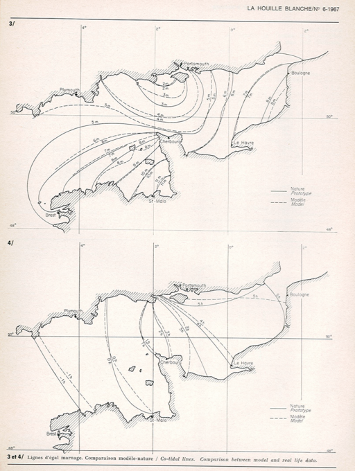
  当前的数值模型能够在1cm的精确度内,模拟重现并预测这些潮汐现象。其中主要的困难是如何量化在湍流条件下海床的摩擦以及激发内潮时的能量损失(参见本文第5节)。

5. 对海平面的其他影响

  潮汐不是影响海平面的唯一因素。首先,我们可以想象一下在通常几米高波浪的海洋中进行厘米测量的可能性。事实上,即便水位波动很大,几平方公里内的平均水位足以很好地代表当地水位。此外,对于图3中的潮汐振幅,仅过滤并保留了给定的时间段(12小时 25分钟),类似于接收无线电波需要选择频率。因此,没有考虑其他频率作用的影响。

  在这些其他影响中,大气压力是相当直接的影响因素。局部高压会降低水位:1 千帕的额外高压通过简单的静力平衡就能使重量为10 3 牛顿/平方米的水柱水位降低10厘米。相反,低压能提高水位。在飓风的中心,大气压为91.3 千帕时,水面能够抬升1 米的高度。这种水位的抬升增强了沿海地区海浪和暴雨造成的破坏。

  另一种破坏是由于风的摩擦力造成的。当它远离海岸时,这股力量使水位降低,反之则将水推向岸边。有暴雨时可以产生约1米高的海浪。这些现象与大潮同时发生能够破坏防御工事,导致洪水泛滥,例如2010年2月袭击法国的辛西娅风暴,或2005年8月袭击新奥尔良的卡特里娜飓风。然而,这些取决于风和大气压的现象比能够导致山洪爆发的局部猛烈降水要容易预测。

  从长远来看,由于海洋扩张,在全球变暖的局势下,平均海平面将继续上升,其中海洋扩张占海平面上升原因的65%,冰川融化占剩余的35%。最近的测量结果表明,海平面平均每年升高2毫米。

  最后,海岸线的水位也取决于地球固体部分的演化。泥沙通过淤积侵蚀改变了海岸线。由于大型河流上的水坝减少了河流中的泥沙输入,因此侵蚀作用目前倾向于占主导地位。由于密西西比河带来的泥沙减少,路易斯安那州海岸受到海水的严重侵蚀。由于几百万年来大陆的漂移,深层地质运动也对海岸线形状的改变有一定影响。在加拿大和欧洲北部,最显著的地质影响就是冰盖融化的地壳反弹,由于10,000年前冰盖的融化,斯堪的纳维亚半岛的沿海水位每年上升几毫米。这种水位升高引起周边地区的下沉(如布列塔尼),譬如7000年前竖立在陆地上的竖石纪念碑如今被淹没在7m深的海水中。

6. 利用潮汐的能量

  自中世纪以来,潮汐工厂就一直在有利的地点利用潮汐能量,如在波涛汹涌的河口或小海湾处修建水坝。1967年投入运行的法国朗斯潮汐发电厂采纳了这个方法,利用了兰斯河口的大坝,以及可在涨潮和退潮时双向运行的定向叶片涡轮机。其总装机容量为240兆瓦,平均运行容量为57兆瓦,发电量占布列塔尼市的45%,供电量占3.5%。投运45年以来,它一直是世界上最大的潮汐发电厂,直到2011年规模更大的韩国四华湖(Sihwa Lake)电厂建成投运(装机容量254兆瓦)。

  但是,有大潮的地点很少允许建造这种规模的设施,并且出于保护自然景观的需要,目前更难临海建立。曾经有一个宏伟的项目拟在潮汐振幅极大的圣米歇尔山(Mont Saint-Michel)建立大坝,但在19世纪70年代遭到放弃,政府转而支持核电发展。

环境百科全书-潮汐-潮汐速度分布图
图6. 潮汐速度分布图和法国布列塔尼海岸的计划安装地点,拉兹·德·塞恩,乌尚和拉兹·布兰查德,插入图片是由EDF开发的潮汐涡轮机模型(直径10米)。

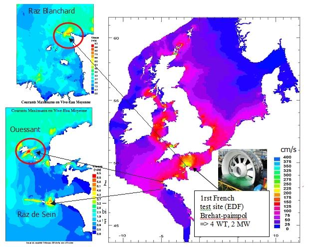
  目前的趋势是直接使用潮汐带动水力涡轮机以及海面上的风力涡轮机,产生电流。这些涡轮机不需要水库,因此对环境的影响较小。但其发展目前仅处于装机容量几兆瓦的初始阶段,仅在苏格兰和布列塔尼设有试点(见图2)。苏格兰的目标是到2020年建成年产1,000 兆瓦的水力发电场。欧洲的总装机容量估计能达到10,000 兆瓦(平均运行容量5,000兆瓦),其中80%位于法国和英国。这相当于法国电力平均消耗量的约10%。

  这一资源仅占潮汐耗散的总功率的0.2%,类比于通过地球自转而消耗的功率(参见第8节)。能源提取趋向于减缓潮流,从而在局部降低其振幅,从而减小粘滞摩擦损失。可以预期,提取的能量将在没有捕获的情况下以热的形式散失。然而,很难计算对地球自转的回馈影响,而这影响非常微小[5]

7. 内潮汐

  海水密度随深度而增加,浅层海水比深层海水温暖(因此密度较小)。这样的密度分层也可能由盐分导致,例如由直布罗陀海峡进入地中海的海水会由于密度较低而停留在浅层水域。这种情况可以总结为不同密度产生的双层模型。

  内部波振荡(通常称海洋内波)可以与表面波相似的方式沿着密度层的分界面传播。然而,受两层之间密度差异的影响,海洋内波的传播速度要慢得多通过用减少的重力gδρ/ρ代替重力g来描述,其中δρ/ω是相对密度两层之间的差异。因此,在厚度为H的表层中,波的传播速度为c=(Hgδρ/ρ)1/2。此时在厚度为100 米的海水表层,内波的传播速度仅为表面波传播速度的1/30倍,约为1米/秒。

环境百科全书-潮汐-苏禄海表面的传播情况
图7. 内潮汐在菲律宾与马来西亚之间的苏禄海表面的传播情况。波浪每12小时产生一次,间隔约100km。(卫星影像来源:http://earthobservatory.nasa.gov/images/3586/internal-waves-sulu-sea)

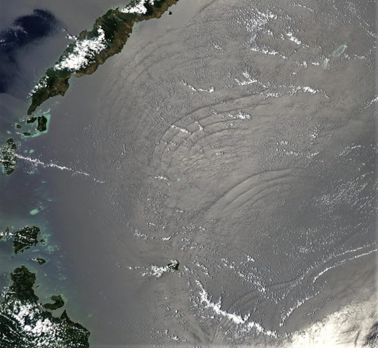
  如图7所示,潮汐在整个水面上引导水平的海流。但是,经过坡面时,该海流会获得一个使界面变形的垂直分量,从而产生一个海洋内波,在这种情况下称为内潮汐。其波长约为100 千米(在12小时的潮汐周期内以1米/秒的速度行进的距离)。而且它们倾向于作为孤立波,位于高振幅的紧凑波中。尽管这些波在深层水域传播,但他们通过传递波形改变海面的亮度,以至于在海洋表面即可观察到其产生的水平海流(图7)。

  在海洋的许多地方都能观察到内潮汐的产生。最活跃的地方之一是位于台湾与菲律宾之间的吕宋海峡,由中国南海的一个水下山脊产生垂直位移超过300米的海洋内波。这些波浪破坏即消散,促进了海水的垂直混合,进而影响了海洋的总体环流气候(参见本文第6节)。

8. 天文效应和能量耗散

  在天文时间上,潮汐以每世纪2毫秒的幅度延长一昼夜的长度推动月球以每年3.8厘米的速度离开。地球自转的减慢目前可以很精确地通过原子钟测量,以2亿年的时间长度衡量,一昼夜的时间大约延长一个小时。地球到月球的距离可以直接通过由阿波罗登月任务发射的反射器所发送的激光脉冲的往返时间测量,测量精度可达1厘米[7]

  对于珊瑚化石的观测证实了地球自转的减慢[6],其环纹圈数可以计量一年的天数。因此,距今4亿年前的每年是410天,每天是21.5小时。根据满月确立的历月数同样表明一年多于13个月,即月亮的旋转速度更快(因此离地球更近)。

  这些影响可以通过图2b的图表理解。地球的自转会使两侧涨潮位置偏移,因此与牛顿静力学模型不一致。来自月球的引力施加了使地球减速的扭矩并为月球带来能量。这样的能量会驱离月球,因而减缓其公转速度(与1 /√r成正比)。然而,由地月之间的距离r和速度相乘所得的月球动量矩却增加(与√r成正比)。地球的动量矩则以相应的比例减小,因此总动力矩保持不变。地月间的总机械能降低,通过潮汐的方式,在洋流过程中转化为热量而耗散。

  天文测量可以精确确定旋转能量的减少,从而推断出潮汐运动消耗的总功率为2.9 ×10 12 W。海洋学家以往估计的功率消耗约为该数值的一半,其中大多数功率消耗在沿海地区。剩下的一半功率,现在可确定为由于激发内潮汐产生的“遗漏耗散”(参见第5节),在海洋深处扩散并最终消散。这种由海浪破裂引起的消散,导致海水的缓慢垂直混合。这些因素对热盐循环的影响正在积极研究中。


参考资料及说明

封面图片:Mont-Saint Michel, où les marées peuvent atteindre un marnage de 15m. source https://upload.wikimedia.org/wikipedia/commons/thumb/2/29/Mont-Saint-Michel_Drone.jpg/1280px-Mont-Saint-Michel_Drone.jpg.

[1] http://www.imcce.fr/promenade/pages5/525.html#Para02

[2] Tidal level records at more than 900 sites over the world are available on http://www.ioc-sealevelmonitoring.org/

[3] Newton I. (1687) ’Philosophiae naturalis principia mathematica’

[4] http://science.nasa.gov/media/medialibrary/2000/06/15/ast15jun_2_resources/oceantides.gif

[5] Maitre T., http://encyclopedie-energie.org/notices/les-hydroliennes

[6] This statement needs to be qualified, as a large energy extraction would in turn change the shape and phase of the tides, and thus the torque exerted on the Earth. nevertheless, a 5,000 MW extraction represents just 0.2% of the total power dissipated in the tides (see section 8)

[7] http://culturesciencesphysique.ens-lyon.fr/ressource/laser-distance-terre-lune.xml

[8] Runcorn S.K. , « Corals as paleontological clocks», Scientific American, vol. 215,‎ 1966, p. 26–33


The Encyclopedia of the Environment by the Association des Encyclopédies de l'Environnement et de l'Énergie (www.a3e.fr), contractually linked to the University of Grenoble Alpes and Grenoble INP, and sponsored by the French Academy of Sciences.

To cite this article: SOMMERIA Joël (March 9, 2024), 潮汐, Encyclopedia of the Environment, Accessed July 27, 2024 [online ISSN 2555-0950] url : https://www.encyclopedie-environnement.org/zh/eau-zh/the-tides/.

The articles in the Encyclopedia of the Environment are made available under the terms of the Creative Commons BY-NC-SA license, which authorizes reproduction subject to: citing the source, not making commercial use of them, sharing identical initial conditions, reproducing at each reuse or distribution the mention of this Creative Commons BY-NC-SA license.