The ensemble forecasting

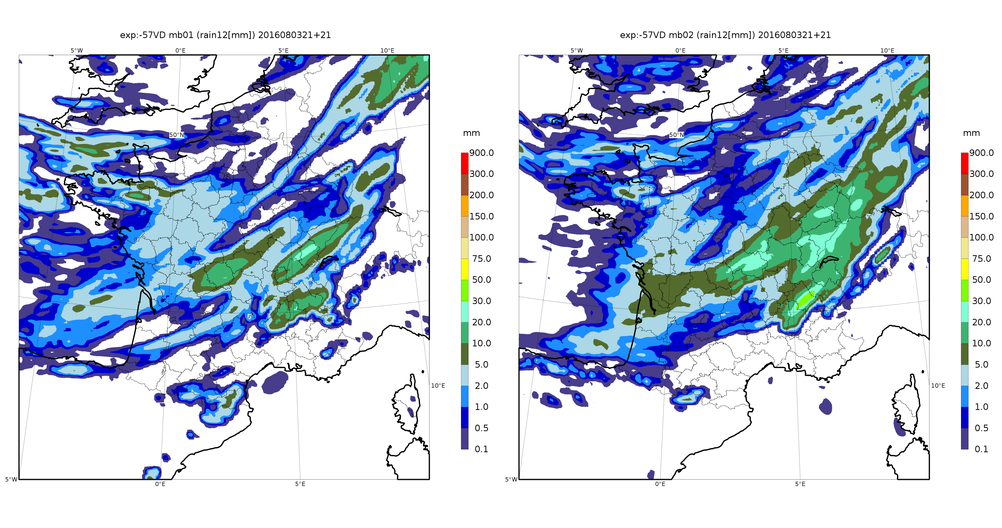
Ensemble forecasting is the tool used to make probabilistic weather forecasts. It is both an alternative and a complement to deterministic weather forecasting that has become essential. It consists of simulating by random drawing the errors made when calculating a numerical weather forecast to arrive at the most probable evolution. These unavoidable errors may result from inaccuracies in the values used to characterize the initial state of the atmosphere, or from approximations made in the equations, or from accepted uncertainties in modelling conditions at the land/air or sea/air interfaces.

1. Interest and principle of ensemble forecasting

Based on observations, a model (for example, a numerical weather prediction model, NWP) (see Introduction to Weather Forecasting) can be used to simulate the evolution of a real system (here, the atmosphere). This produces the best possible estimate of the future, called a deterministic forecast: the best data are then used to make a single forecast. Everyone can see that in practice, this forecast is often imprecise, due to the lack of initial observations, their errors, and the approximations made during the numerical simulation. In addition, weather forecast errors frequently increase due to the chaotic nature of the atmosphere: it is the butterfly effect, whereby a small error in the data or model can make the forecast completely wrong a few hours or a few days later. For a forecast to be useful, it must be better than a trivial forecast, less costly to obtain, for example a weather report that would simply state seasonal normals as a forecast. The time scale beyond which we generally do not know how to make a useful forecast is called the predictability horizon. This horizon is currently, on average, a few minutes for a shower, a few hours for a storm, a few days for a depression or cyclone, a few weeks for a cold or heat wave, a few months for a tropical climate anomaly such as El Niño.

This horizon, and more generally the quality of the forecasts, are highly variable in space and time. It is therefore interesting to know precisely how much confidence one can have in each of the aspects of a forecast: this is the objective of probabilistic forecasting, where a range of possible forecasts is produced. Since it would be numerically very expensive to calculate all possible alternatives, the problem is approximated by replacing the calculation of a deterministic forecast with that of a few randomly disturbed numerical forecasts: this is the ensemble forecast. These forecasts are made in real time, as would a deterministic forecast. If we have n forecasts (called members), all their forecasts for a given meteorological parameter x (for example, the wind speed at a given point at a given time) are made up of n values, which mathematically constitute a discrete sample of the probability density [1] of x, taking into account the data available at the time the forecast was run. Section 3 shows that ensemble forecasting produces not only parameter probabilities, but also a full range of meteorological scenarios, physically coherent in space and time. It is therefore a very rich source of information, the proper use of which is a challenge in its own right.

The notion of predictability horizon has been popularized in meteorology by Lorentz [2], whose explanation of the chaotic processes involved by the image of the butterfly effect has left its mark on the general public. The first real-time operational ensemble forecasts are due to Toth and Kalnay [3], using the American meteorological model. Since then, ensemble prediction technology has been perfected and applied in all major weather services (Leutbecher and Palmer [4]), both for the prediction itself and for data assimilation. It has also spread to other sectors, such as numerical simulation for industry, finance, hydrology, seasonal forecasting [5] (see The Seasonal Forecast), etc.

From an operational point of view, making an overall forecast consists in executing a numerical prediction software n times, disturbing by random numbers its input data as well as the calculations of the software itself. These disturbances should ideally reflect the distribution of our uncertainties over all these data (e.g. observational errors) and calculations (e.g. meteorological processes that are known to be poorly modelled, such as ocean surface flows). This makes it possible to simulate different possible evolutions of all these errors within the forecast model and their impacts on the predicted parameters. Parameters affected by large errors, or by a chaotic amplification of disturbances, will have more scattered forecasts than parameters whose prediction remains stable despite disturbances: the dispersion of ensemble forecasts thus provides us with information on the predictability of phenomena simulated by the numerical model (Figure 1).

2. How to disrupt a weather forecast?

In practice, only some key aspects of numerical prediction systems are disrupted because our knowledge of the sources of errors is very limited. In the current state of the art, the disturbances concern:

• The initial state of the forecast. The aim is to represent the uncertainties of the analysis process, mainly related to observation errors and defects in data assimilation algorithms. The simplest technique consists in adding to the deterministic analysis a numerical noise [6], for example Gaussian, with spatial correlations and amplitudes faithful to the statistics carried out on past analyses. This noise can also be constructed by linear combinations of differences between recent analyses or forecasts (LAF method: lagged averaged forecasting). A common method is to add optimized disturbances to the analyses in order to amplify as quickly as possible during the ensemble forecast. This ensures that the whole will simulate the effect of the main sources of chaos of the day. A more rigorous, but also more expensive, method is to calculate sets of the complete data assimilation process (see Assimilation of meteorological data): these are the ensemble assimilation methods, or the ensemble Kalman filter methods.
• The equations of the forecast model. It is about representing modeling errors. This can be done by mixing several versions of the numerical model of the atmosphere (the multimodel method) into the ensemble prediction, or by varying certain key parameters whose optimal value is poorly known (multiparameter method), or by injecting random disturbances into certain parts of the code that are known to be suspect (stochastic physics method). The difficulty is that most modelling errors are by definition unknown, since they come from meteorological processes that may be unknown; there is therefore a lack of information to simulate them. Some sources of errors have been particularly studied, such as the presence in the real world of unresolved physical scales due to the limited resolution of the numerical model; they can be simulated by using fictitious energy sources in ensemble forecasts (stochastic energy backscatter method).
• Surface conditions. The interaction between atmosphere and surfaces is a major source of forecast errors. This is often due to the representation of physical parameters by artificially fixed values during weather forecasting, because we do not know how to correctly represent their variability. It is therefore necessary to represent their uncertainties in a specific way, by disturbing them in a way that is consistent with what we know about their uncertainty. This concerns in priority the characteristics of the soil, vegetation, snow, oceanic properties determining the calculation of temperature flows, humidity and turbulence. In the most sophisticated assemblies, the surfaces themselves are complete numerical models from which predictions of systems coupled with the atmosphere can be made. This is particularly the case in seasonal forecasting.
• Large-scale couplings. This only applies to digital models with a limited domain. Their predictions are sensitive to errors in the global weather model to which they are coupled, which is crucial to predict the evolution of large, rapidly propagating atmospheric waves. The limited area ensemble forecasts must be coupled with global ensemble forecasts that realistically represent the uncertainties of large-scale atmospheric evolution.

3. From ensemble forecasting to applications

The ensemble forecast produces rich and often difficult to understand information. From a mathematical point of view, an ensemble forecast produces different possible scenarios of atmospheric evolution. Since the dimension of the space in which the atmospheric state evolves (several billion degrees of freedom) is much larger than that of the ensemble forecast (a few dozen members), the latter only provides an overview of possible evolutions. There are different methods of interpreting ensemble forecasts, the main ones being as follows.

• The subjective examination of ensemble forecasts allows a trained forecaster (see The Role of the Forecaster) to estimate the likelihood of different possible forecast scenarios. In general, he/she will look at a super ensemble of forecasts consisting of all recent model outputs (set or deterministic) available at the time he/she is asked to interpret the forecast. Modern forecasters have access to a large number of very likely forecasts, from different weather centres, different models, or calculated at different times: they always reason probabilistically, whether they use or name real ensemble forecasts. Most forecasters prefer the consensus scenario, i.e. the one supported by the majority of models and members; forecasts that are too atypical are then rejected as too unlikely to merit mention in the bulletins. However, if some forecasts indicate the possibility of a hazardous event occurring, this can help to issue a weather warning, if necessary by taking the risk of issuing a false alarm, given the potential severity of the event. Ensemble forecasts can be useful in estimating uncertainty about the intensity, location or timing of weather events, and this allows them to be predicted with greater confidence than if only deterministic forecasts were available, knowing that this requires a specific effort on the part of the forecaster [7].

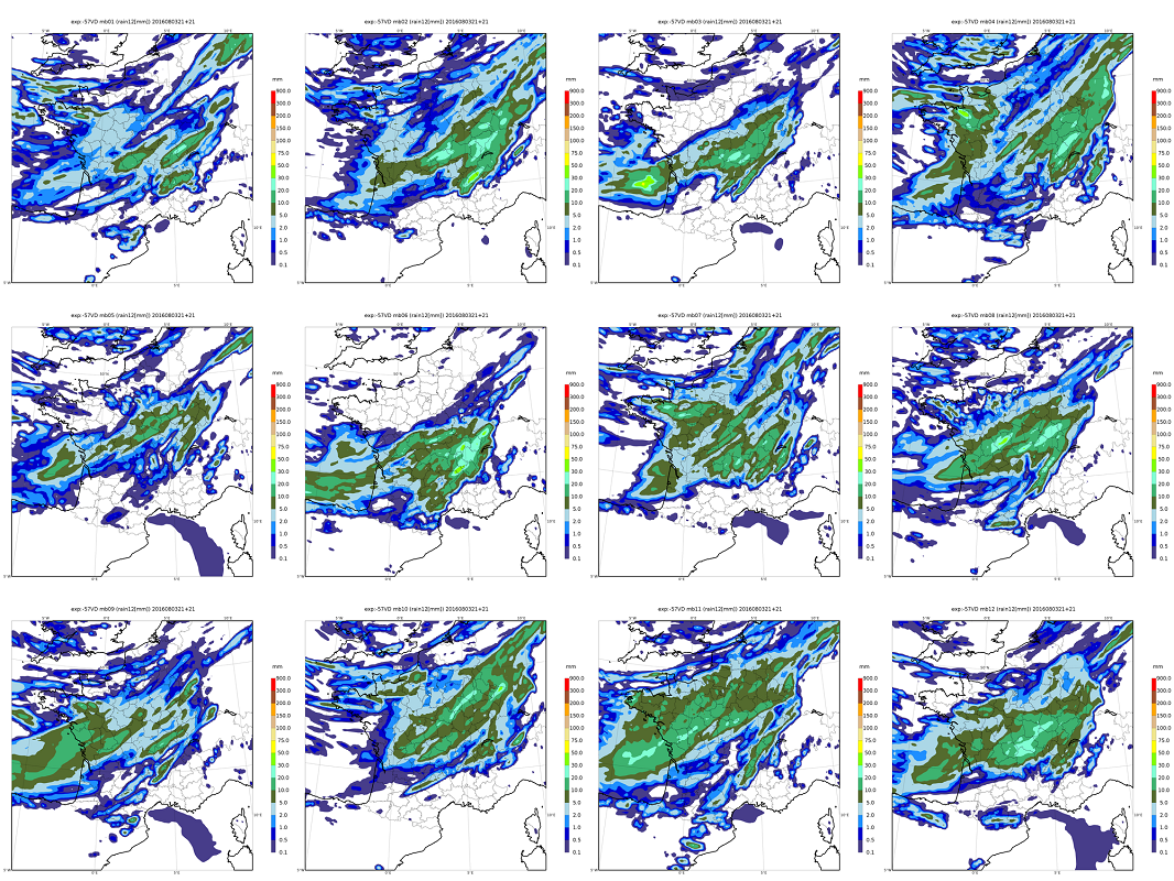
• The production of automated forecasts is more efficient (i.e. more accurate) if it is based on sets than on deterministic forecasts alone, for the same reasons as above. Indeed, the sets provide rich information, which makes it possible to process forecasts in a sophisticated way. These treatments often mimic the work of human expertise in forecasting. For example, the distribution of predicted values of a meteorological parameter at a grid point in the model is an estimate of the probability distribution of that parameter; at each point there are as many values as there are members overall (see Figure 2). These values can be corrected by statistical processing to compensate for systematic defects in the numerical model, such as biases in the forecast values, or too much confidence in the forecast (represented by too little dispersion of the set compared to errors found in recent forecasts). Users can be provided with the median value predicted by the set, which is usually a very likely value. But we can do better, by using the range of probabilities calculated by the ensemble; for example, a user who accepts 3 times more false storm alerts than no detection (which is, consciously or unconsciously, the case for most users in the general public) will perceive far fewer forecast failures if he is warned of the risk of a storm from the probabilities of a ensemble greater than 25%, than if he were given the median forecast, or that of a deterministic model. It is in applications where the false alarm rate tolerated is very different from 50% that the overall forecast provides the greatest improvement in weather forecasting. This way of using forecasts is similar to the calculations of a financier who seeks to minimize his losses according to the hazards of the economic context: the ensemble forecast applies this approach to concrete weather problems, thanks to a numerical forecast processing adapted to the needs of various types of users.
• Coupling of the overall forecasts. Summarizing the scenarios of an ensemble forecast by probabilities of weather variables often results in a loss of information; in some applications, it is better to directly couple the numerical outputs of the expected members to the complex calculations specific to that application. This is particularly true for applications that are sensitive to the spatial distribution of meteorological variables: flood forecasting depends on integrated rainfall at the watershed scale, routing of commercial aircraft depends on the time encountered along the trajectories of each aircraft, electricity grid management depends on the mapping of wind and photovoltaic production and domestic heating, etc. In these cases, it is up to the application model manager to transform the weather ensemble forecast into an ensemble forecast for his own parameters of interest, which can be influenced by non-meteorological factors. This working method is primarily aimed at professional users, as they must themselves be experts in the use of numerical weather forecasts and probability calculations.

4. What is an ensemble forecast worth?

If rain was forecast with a probability of 50% and it does not rain, was the forecast good or bad? On an isolated case, it is impossible to answer: a probabilistic forecast is never intrinsically good or bad. To assess its quality, it is necessary to carry out statistics on a forecasting history, which can be problematic for the study of rare phenomena. As mentioned above, the very use of an ensemble forecast depends on the user, in particular on his tolerance for false alarms. To take the example of the previous section, a user interested in storm probability forecasts of 25% (adapted for example to the organization of a picnic) will have a very different perception of the performance of a forecasting system than a user who is looking for probabilities of 80% (such as a tornado hunter). These two factors (need for long statistics, and diversity of users) explain why the quality measurements of ensemble forecasts are made with rather complex mathematical tools. By simplifying, we can distinguish 3 main categories of quality measures from forecasts that are relevant for ensemble forecasts:

• Reliability is the consistency between predicted probabilities and observed statistics when comparing forecasts with observations a posteriori. A basic measure of reliability, the dispersion/error relationship, is the correlation between (a) changes in the dispersion of a set, and (b) changes in the amplitude of forecast errors: in a reliable system, the most dispersed forecasts are on average the worst, so this correlation should be as high as possible. We can also look at whether, when a given probability value is predicted, the forecast errors found are consistent with that probability. Example: on an ensemble of cases where rain has been forecast with a 50% probability, rain must be observed in 50% of these cases. Reliability measurements can detect some shortcomings in overall forecast systems, but unfortunately they do not guarantee that the forecasts produced are useful: they do not measure the extent to which forecasts vary from one situation to another, which is necessary to communicate information adapted to each situation.
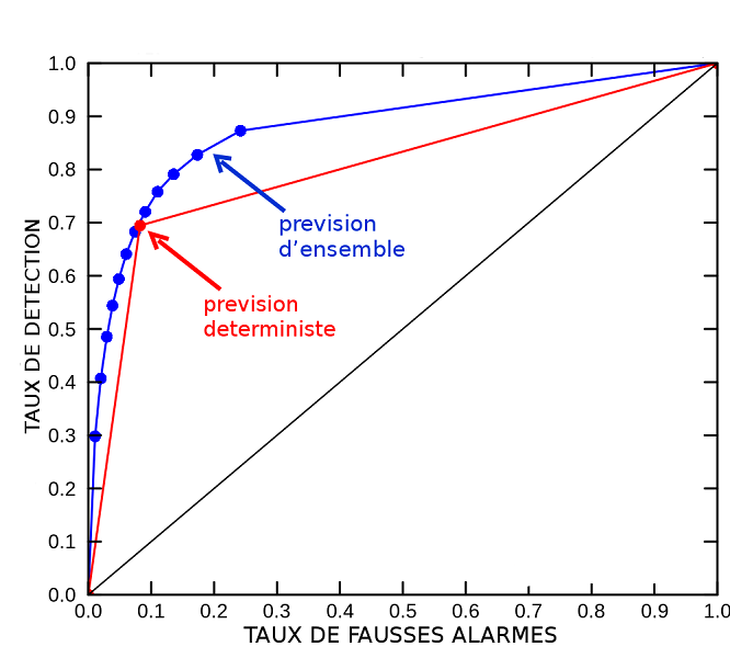
• Statistical resolution, also called sharpness or resolution, is a type of diagnosis that measures how substantially different the predicted probabilities are from climatology (i.e. whether the ensemble is “taking risks”) and then what their average accuracy is. The most common tool is the ROC (receiver or relative operating characteristic) diagram, which measures the success rates of forecasts for all expected probability levels (i.e., on average over a wide range of possible users). The ROC is very useful for assessing the intrinsic performance of an ensemble forecasting system (The role of the forecaster) (see Figure 3).

• Decision value (also called economic value for historical reasons) measures the value of a forecasting system for a specific type of user, whose weather sensitivity is often modelled by (a) the threshold value of a weather parameter to which he or she is sensitive, and (b) the relative cost he or she attributes to false alarms and non-detections of this threshold exceedance. It is within this framework that the value of ensemble forecasts can be most rigorously quantified, and in particular what they contribute in relation to deterministic forecasts [8]. This approach requires a specific work of dialogue with the user to correctly model his weather-sensitivity.

A fourth obstacle that any forecasting system must overcome is the understanding of information by users. Although the current ensemble forecasts are far from perfect, they contain a very high decision value for many uses. Unfortunately, they often suffer from misunderstanding on the part of users, who often prefer more rudimentary but easy-to-understand forecasting tools. The greatest current challenge in ensemble forecasting will be the development of automated processing of the information produced by ensembles, in order to present it in a form that is both intelligible and as accurate as possible.

 

---

References and notes

Cover image. Rainfall forecast over France on August 4, 2016 using the ensemble forecast.

[1] Probability density is a function that mathematically describes the range of possible values that a parameter can take.

[2] Lorentz, E. N. 1963: Deterministic nonperiodic flow. Journal of Atmospheric Sciences. 20 : 130-141.

[3] Toth, Z., and E. Kalnay, 1993: Ensemble forecasting at NMC: The generation of perturbations. Bull. Bitter. Meteor. Soc., 74, 2317-2330.

[4] Leutbecher, M., and T. N. Palmer, 2008: Ensemble forecasting. J. Comp. Phys. , 227, 3515-3539.

[5] Hagedorn, R., F. J. Doblas-Reyes, and T. N. Palmer, 2005: The rationale behind the success of multi-model ensembles in seasonal forecasting–I. Basic concept. Tellus, 57A, 219-233.

[6] Correlations of a noise measure the relationship between its value at one point, and its values at neighbouring points.

[7] Novak, David R., David R. Bright, Michael J. Brennan, 2008: Operational Forecaster Uncertainty Needs and Future Roles. Wea. Forecasting, 23, 1069-1084. doi: http://dx.doi.org/10.1175/2008WAF2222142.1

[8] Climatology refers to the statistical distribution of weather situations observed in the past.