Diffusion, the ultimate step in a good mixture
PDF
Chemical species such as carbon dioxide (CO2) in the air, or sugar in coffee, end up, after a while, being intimately mixed with the surrounding fluid, even if it is at rest. The same mechanism transports heat through the stationary bodies until their temperature is uniform. Similarly, in a fluid layer subjected to friction, the force exerted on the surface is transmitted in its full thickness. In fluid environments, turbulence disperses the constituents, but does not reach molecular scales; it is the disordered agitation of molecules that completes this transport process called diffusion. We will see that it alone would be extremely slow but that turbulence helps it effectively.
The word diffusion is used with relatively varied meanings. What is common to all situations is the fact that a certain quantity is transported through a medium dispersed by the agitation of the elementary particles that constitute it. In physics, we distinguish two families of diffusion phenomena:
- A transport phenomenon based on the properties of the medium under consideration, consisting of atoms or molecules in disordered agitation. It is characterized by the fact that the distribution of the transported quantity tends to become uniform; this quantity may be the concentration of a particular chemical species, heat or the amount of movement. The uniform end state is the thermodynamic equilibrium of the environment.
- The phenomenon of diffraction of waves in a non-homogeneous environment, whether these waves are electromagnetic like light or acoustic like sound. These phenomena are described in other articles in this encyclopedia: The Colours of the Sky, Emission, Propagation and Perception of Sound. In the English language, this phenomenon of wave diffraction is referred to as scattering, which distinguishes it from diffusion itself.
In everyday language, the same word, diffusion, is used with even different meanings. Thus, it can refer to the transfer of knowledge to a large number of people; it can also refer to the transmission of various types of information by radio (called radio broadcasting) or television (called television broadcasting).
- 1. The air at rest: an agitated set of molecules
- 2. Molecular parameters with macroscopic properties of a gas, or the reverse
- 3. The mechanism of diffusion in gases
- 4. The turbulent diffusion
- 5. Mass and thermal diffusion
- 6. Diffusion of movement: viscosity
- 7. The mechanism of diffusion in liquids
- 8. Messages to remember
1. The air at rest: an agitated set of molecules
In the article The Earth’s Atmosphere and Gaseous Envelope, the main components of dry air are mentioned: nitrogen (71%), oxygen (28%), argon (less than 1%), as well as some other gases in much smaller proportions. This set is made up of molecules, which occupy all the available space, a specific property of gases, which distinguishes them from the condensed states of matter (liquid or solid). These have their own volume, the solids also having their own shape.
2. Molecular parameters with macroscopic properties of a gas, or the reverse
It is quite simple to link these parameters of the molecular world to some macroscopic quantities, measurable and accessible to our senses. These quantities – analyzed in the article Pressure, Temperature and Heat – are pressure p, temperature T, mass of the volume unit (or density) ρ and viscosity [3] μ For this purpose, we have an almost obvious first relationship between molecular and macroscopic scales: mass m is the quotient m = M/NA between the molecular weight M and the Avogadro number (number of molecules per mole) NA = 6.022×10²³ mol-1. In addition, the density ρ must be equal to the product of the number n of molecules present in the volume unit multiplied by the mass of each molecule. We therefore have a second relationship between the parameters of the two worlds: ρ = nm.
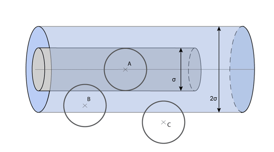
To connect the pressure p at a point in the gaseous medium to its molecular parameters, let us imagine that a flat solid surface of unit area (S = 1, whatever the chosen system of units) is placed somewhere in this gaseous medium. Each of the two sides of the surface will receive and accumulate the impulses of all the molecules that will hit it during the unit of time, coming from all directions, losing and regaining their kinetic energy, in the order of mc2/2 for each of them. On average, the force exerted on the unit surface and equal to p must therefore be of the order of nmc2. A rigorous calculation, taking into account the real velocities of the molecules encountered [4], would lead to the expression p = nmc2/3. In passing, we obtain an evaluation of the error due to the simplifying assumptions of the model adopted: the coefficient 1/3. The important thing here is that we have obtained a third relationship between the molecular parameters (n, m, c) and a macroscopic property, the pressure p.
Since pressure and density are related to molecular parameters, it is sufficient – to express temperature – to identify the pressure p expressed above with the one that verifies the state equation of perfect gases: p/ρ = RT/M, where R = 8.314 m3.Pa.mol-1.K-1 denotes the universal constant of perfect gases and M the average molar mass of the gas mixture. We obtain the fourth relationship [5] T = Mc2/3R which highlights the proportionality between the temperature T and the square of the velocity of the molecules c2 (Read Pressure, Temperature and Heat).
To these four relationships should be added the one that expresses the dynamic viscosity of the gas, which is established later in Section 5: μ = nmcλ/3. So, with the following values, common for sea-level air
p = 1.013 105 Pa, T = 288 K, ρ = 1.22 kg.m-3, ν = 10-5 m2.s-1,
the five relationships mentioned above lead to:
n = 2.5 ×1025 m-3, m = 4.8 × 10⁻²⁶ kg, c = 497 m.s-1,
d = 3.4 × 10⁻⁹ m, σ = 0.46 × 10⁻⁹ m, λ = 6 × 10⁻⁸ m.
To get a fairly accurate idea of the scales of the molecular world, we can see that the number of molecules contained in a small cube of one micron on each side is about 25 million. We will deduce that the typical distance between two neighbouring molecules (d) is about 7 times their diameter (σ), that their average free path (λ) is about 60 nanometers, or about 130 times their diameter, and that the average speed of the molecules is slightly higher than the sound velocity (340 m.s-1).
3. The mechanism of diffusion in gases

However, the time required to establish this balance is much longer (hours or more) than the time between two molecular collisions (in the order of λ/c ≈ 1.4×10⁻¹⁰ s). Under these conditions, collisions are so frequent around a given point that it can be assumed that molecules that leave the vicinity of that point after a collision all carry the same value of G, i.e. G/n since G refers to the value per unit volume. It is then said that this gas is in a state of local equilibrium.
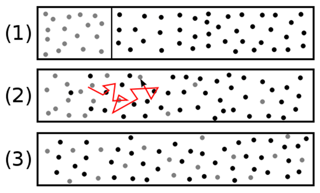
Molecules that pass through a flat surface unit perpendicular to the x direction (back to Figure 3) have, on average, the size G/n. The distance from where they come is in the order of an average free journey λ. The smallness of this length λ compared to the macroscopic dimensions justifies assuming linear, with a slope Γ0, the distribution G(x) in the vicinity of the cut located at x = 0. This leads to the simple distribution: G = G0 + Γ0 x. Let’s even assume that the molecules that come from the x>0 side all carry G+ = G0 + Γ0λ, and that those that come from the x<0 side carry G- = G0 – Γ0λ.
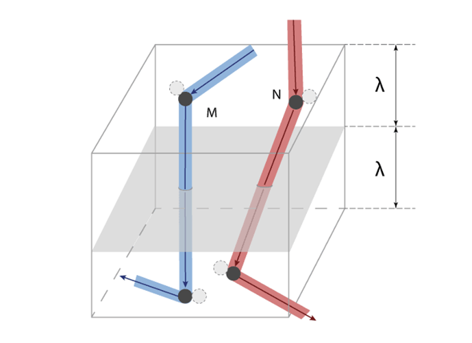
Finally, the flow rate φ of G through each unit of surface of the plane x = 0 can be estimated by the relationship φ = (cλ/3) dG/dx. The conclusion of this estimate is as follows: if a quantity G is distributed non-uniformly, the net flow of G transported by molecular agitation is proportional to the local gradient dG/dx and is expressed by a relationship of the form φ = -D dG/dx, where, by convention, the sign is placed – so that the flow is positive when dG/dx is negative (heat goes from the warm side to the cold side). The coefficient D appearing in this relationship is D = cλ/3. It is called the diffusivity of this gas; it is a purely kinematic quantity measured in m2/s. It is remarkable that it was possible to assess the diffusivity of the gas without specifying the nature of the size transported.
The numerical values given in section 2 are used to estimate air diffusivity. With c = 497 m s-1 and λ = 6 × 10⁻⁸ m, we obtain : D ≈ 10-5 m2 s-1. To give this value a practical meaning, let us return to the experience in Figure 4: If we note L the length of the enclosure, since diffusivity has the dimension of a square length divided by time (L2T-1), the typical duration to reach the final state in equilibrium is necessarily in the order of L2/D. If L ≈ 10 cm, this duration is about one hour. For this duration to be in the order of a second, the enclosure in Figure 4 would have to be about a millimeter long, as would be the case with a small bubble.
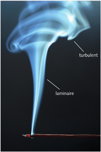
4. The turbulent diffusion
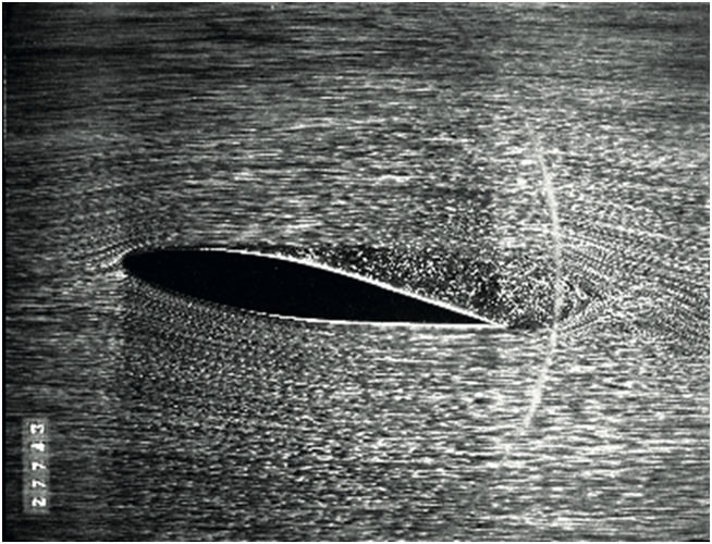
In most of the fluid environments in our environment, including air and water, turbulence is almost omnipresent. It is a phenomenon of agitation totally unrelated to the movement of molecules. Within a flow such as the wind, or as a marine current, it manifests itself in the presence of large scale, fairly large and easily measurable speed fluctuations. Even without imposed flow, in the presence of hydrodynamic instability [ 6], turbulence is present as a set of vortices of all sizes entangled in each other. We can see a certain analogy with the molecular agitation described in the previous sections, but at the vortex scales, much larger than the average free path of the molecules. This analogy led Prandtl[7] to suppose that it was possible to define a mixing length [8], similar to the average free path of the molecules of a gas.
The concept of mixing length, size noted below, is rather vague but it has the merit of allowing satisfactory orders of magnitude to be established. The situation where it is best justified is that of a boundary layer (see Figure 7). The expression suggested by Prandtl in such a boundary layer and generally adopted is l = κy, where there is the distance to the wall and κ a numerical constant determined by experience. With this expression of the length l, the order of magnitude of the velocity fluctuations at the distance y from the wall can be estimated by u’ ≈ l dU/dy. The analogy with gas agitation suggests reusing the expression of molecular diffusivity (D = cλ/3) by replacing c by u’ and λ by l = κy. The turbulent diffusivity Dt within a boundary layer then becomes: Dt ≈ u’l ≈ κ2y2 κ2y2 dU/dy.
For example, let us place ourselves within the atmospheric boundary layer, whose thickness is about a few hundred meters, at a distance from the ground y ≈ 10 m where the average speed is about 10 m.s-1 and where dU/dy ≈ 1 s-1. By adopting the value 0.1 for the constant κ, derived from experiments, these estimates lead to a turbulent diffusivity Dt ≈ 10 m2.s-1, i. e. one million times higher than the molecular diffusivity. This value reduces the time required to achieve the turbulent mixture to about one-tenth of a second: t ≈ l2/Dt ≈ 0.1 s. But this mixing is not complete because the components are only dispersed to the scale of the smallest vortices, which depends on the viscosity of the fluid. In the case of the atmospheric boundary layer, it is about one millimeter. It is the molecular agitation that completes the mixture to the molecular dimensions, and we know that this requires an L2/D duration. In reality, molecular scattering begins within millimetre eddies where it coexists with turbulent dispersion. To simplify, let us assume that molecular scattering acts alone below the millimeter. With L ≈ 10-3 m and D ≈ 10-5 m2 . s-1, we still obtain a duration of about one tenth of a second.
From these estimates, it can be concluded that:
- the turbulent diffusion only disperses the constituents to the scale of small eddies,
- molecular diffusion completes this mixture,
- the durations of the two mechanisms can have orders of magnitude in the order of one tenth of a second,
- without turbulence, the time required to make a good mixture could reach several hours.
5. Mass and thermal diffusion
It is by the expression mass diffusivity that we usually refer to the diffusivity of a chemical species contained in the fluid medium. Suppose, therefore, that some of the molecules of the fluid considered, gas or liquid, are different from the others. Let’s take the example of water molecules (H20) in the form of steam, in absolutely calm air over a large liquid area, such as a peaceful lake. And let us now note C the volumetric concentration of water in the air at any altitude z, a quantity initially noted as G before its nature was specified. To evaluate the net flow of water vapour to high altitudes, the law seen above leads to the expression φ = -D dC/dz. It’s Fick’s law. It is essential to be able to calculate the quantity of water extracted by diffusion from low altitudes, but it must be supplemented by a mass balance and by initial and boundary conditions.
Thermal diffusivity expression is reserved for heat transport by molecular agitation. Let us now assume that quantity G is the internal energy E per unit volume of the gas, any infinitesimal variation of which is manifested by a temperature variation dT, according to the law dE = ρCv dT, where Cv denotes the constant volume calorific capacity of the gas. Then the diffusion transport of this internal energy, i. e. heat, becomes φ = -ρCvD dT/dz. It is common to write this expression called Fourier’s Law in one of the following two forms: φ = -k dT/dz, where k = ρCvD = Cv nmcλ/3 is called the thermal conductivity of gas, or φ = -α ρCp dT/dz, where α = k/ρCp is the thermal diffusivity of gas. The quantity Cp then refers to the heating capacity at constant gas pressure.
The physical properties of the gases, especially air, introduced above (D, k, α, μ, ν) are related to the molecular parameters n, m, c and λ. Among them, for a given density gas, only the velocity of molecules c is likely to vary with temperature T. And we saw that this dependence could be written: T = Mc2/3R = mc2/3kB. It can be deduced that the diffusivities of a gas (D, k, α, μ, ν) vary like the square root of its temperature.
6. Diffusion of movement: viscosity
Let us now assume that the above notions remain valid in a fluid set in motion at macroscopic scales by moving a wall in its own plane. This hypothesis is very well justified as long as the typical durations of macroscopic motion (seconds or minutes, in general) are considerably longer than the time between two collisions of a molecule (about 10-11 s).
The above reasoning also applies when, instead of being materialized by a wall, the plane z = 0 is an interface between two fluid layers, one of which is moving in its own plane, at the velocity u, between the fluid above it and the fluid below. Newton’s law thus makes it possible to express the tangential force, often called friction, that the fluid layers exert on each other. This tangential force, oriented in the velocity direction, is added to the pressure force, which is oriented according to normal at the interface (Read Pressure, Temperature and Heat).
7. The mechanism of diffusion in liquids
The fact that all liquids have their own volume implies that the molecules that compose them are close to each other. The average distance between neighbouring molecules depends on the pressure exerted on this liquid; under normal conditions (p ≈ 103 hPa) it is slightly larger than the size of the molecules, typically 10-10 to 10-9 m. The thermal agitation of all these molecules, which can be compared to a vibration, gives this liquid medium a certain diffusivity, but this is much lower than that of gases. The difference is essentially due to the fact that, in a liquid, the radius of action of a molecule is less than its size, whereas in a gas, it is the average free path, about 25 times the size of the molecules. This weakness explains why, in order to dissolve the sugar in a cup of coffee, it is necessary to add a macroscopic stirring by stirring the whole with a spoon.
Any particle with a difference from the molecules and present in this medium is constantly subjected to the vibrations of the whole. A balance similar to that for gases in section 3 necessarily shows a net flow of these particles from the richest to the poorest side. This flow rate can still be written with Fick’s law: φ = -D dC/dx, where D denotes the diffusivity of the particles in the liquid and C their volume concentration.
To predict the mass diffusivity of a liquid, which reflects its ability to transport another material species, we have the following law proposed by Einstein in 1905[11] : D = kBT/6πμr, where kB = 1.38×10⁻²³ J.K-1, is the Boltzmann constant, T the absolute temperature, μ the dynamic viscosity of the liquid and r the radius of the transported particle. With r ≈ 10-9 m, in a liquid such as water or μ ≈ 10-3 Pa.s, at an ambient temperature close to 300 K, we obtain D ≈ 2×10⁻¹⁰ m2.s-1, a value about 10 000 times lower than the diffusivity of a gas. In Einstein’s formula, we will notice that T intervenes at the numerator, which reflects the fact that thermal agitation is the real driving force behind diffusion. And the fact that μ and r are involved in the denominator means that viscosity is opposed to diffusion and that the larger the particles, the more difficult it is to diffuse.
For water and for any electrically insulating liquid, heat and mass have similar diffusivities. On the other hand, for liquid metals, electronic conduction is another heat transport mechanism that can be much more important than mass diffusivity. The most well-known example is liquid sodium, used to cool nuclear reactors of the superregenerator type such as Phoenix, which operated at Marcoule from 1973 to 2010. Its thermal diffusivity at a temperature of about 300 K is about 7×10⁻⁵ m2.s-1, more than 10,000 times higher than its mass diffusivity.
8. Messages to remember
- The diffusion of a particular species within a mixture, like the diffusion of heat and the diffusion of the amount of movement, results from the agitation of elementary particles, molecules or atoms. It is a very slow transport mechanism, but without a competitor on microscopic scales.
- In fluids such as air and water, which are not very viscous, turbulence disperses pollutants, heat and the amount of movement. But this mechanism cannot reach scales lower than those of the smallest vortices, controlled by viscosity, generally greater than one micron. Molecular diffusion relays it to complete the mixture.
- The laws of diffusion were first discovered empirically before being the subject of theoretical models. Relatively simple in the case of diluted gases such as air, it could be sketched in this article. Its equivalent in the case of liquids is much more complex and still under investigation.
References and notes
Cover image. Before sunrise, in the countryside, in the still motionless air, it is by diffusion that contaminants released by vegetation are transported into the air. [Source: pixabay, royalty-free].
[1] A nanometre is one billionth of a metre (10-9 m), a micrometre, or micron, is one millionth of a metre (1 μm = 10-6 m).
[2] Ludwig Boltzmann (1844-1906), an Austrian physicist and philosopher, introduced this molecular model called “hard spheres” that leads to a famous equation bearing his name.
[3] It is often substituted by the kinematic viscosity ν, which is the quotient between the viscosity μ and the density ρ, i.e. ν = μ/ρ.
[4] All these velocities, with their respective orientations and values, can be represented using Maxwell’s distribution function. Taking them into account would lead to lengthy calculations beyond the scope of this article.
[5] This expression is better known as kBT = mc2/3, by introducing the Boltzmann constant kB, related to R and the Avogadro number NA = 6.0248 × 10²³, per kB = R/NA= 1.380 × 10⁻²³ J/K (joule by Kelvin).
[6] For example, at dawn, as soon as the sun begins to warm the ground, by diffusion it heats the lowest layers of air, which become lighter than those above them. This situation where the heavy fluid is located above the light fluid is unstable.
[7] Ludwig Prandtl (1875-1953) was a German physicist, professor at the University of Munich, who made important contributions to fluid mechanics. He is credited with the founding ideas of boundary layer theory, the concept of mixture length and a simple theory for calculating the lift of a finite wing span.
[8] M. Lesieur, Turbulence, EDP Sciences, Grenoble sciences collection, 2013, p. 128.
[9] The property that φ = -τ can be established by writing the global equilibrium of a small gas domain located on the z>0 side of the wall that exerts the tangential force on the fluid -τ. The expression of this global equilibrium is often referred to as the quantity of movement theorem.
[10] The establishment of this expression is actually due to Navier, Fourier’s congener (see the focus on the Fathers of the diffusion concept).
[11] Albert Einstein, Investigations on the Theory of the Brownian Movement, Dover Publications, Inc. (1985), (ISBN 0-486-60304-0). Reissue of Einstein’s original articles on Brownian motion theory
The Encyclopedia of the Environment by the Association des Encyclopédies de l'Environnement et de l'Énergie (www.a3e.fr), contractually linked to the University of Grenoble Alpes and Grenoble INP, and sponsored by the French Academy of Sciences.
To cite this article: MOREAU René (January 5, 2025), Diffusion, the ultimate step in a good mixture, Encyclopedia of the Environment, Accessed July 27, 2026 [online ISSN 2555-0950] url : https://www.encyclopedie-environnement.org/en/physics/diffusion-ultimate-step-good-mixture-2/.
The articles in the Encyclopedia of the Environment are made available under the terms of the Creative Commons BY-NC-SA license, which authorizes reproduction subject to: citing the source, not making commercial use of them, sharing identical initial conditions, reproducing at each reuse or distribution the mention of this Creative Commons BY-NC-SA license.