How matter deforms: fluids and solids

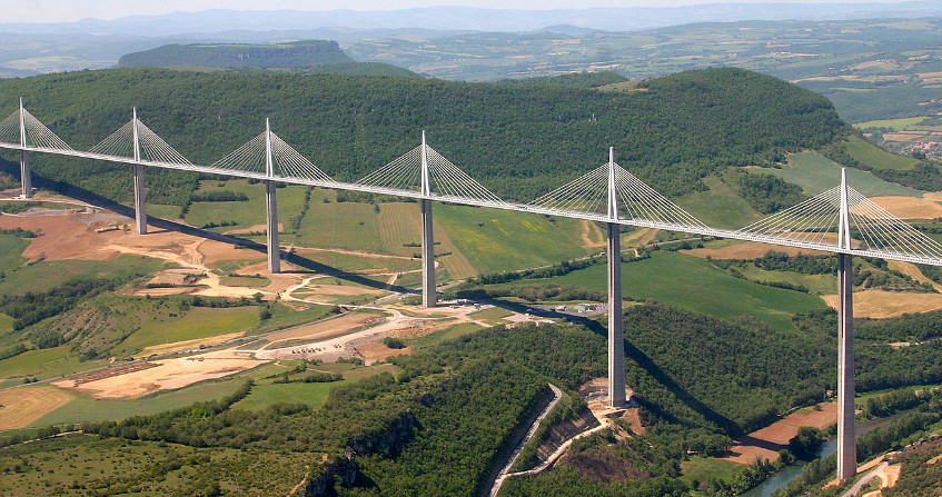
An ice cube in a glass is a fragile elastic solid, but the Sea of Ice in Chamonix flows like a viscous fluid. Indeed, any material can change from solid to fluid behaviour, and vice versa, under the effect of mechanical or thermal stresses. But how can we describe these two states of matter and the associated behavioural classes: elasticity, viscosity and plasticity? Why are new variables, stresses and strains, needed to describe the internal stresses and strains of the material? What are the relationships that link stress and strain between them? Why does the calculation of structures or structures require the use of such relationships? This is the purpose of this article.

1. Fluids and solids

There are classically three states of matter: gases, liquids and solids. But other, more complex states also exist, such as pastes, gels and plasmas, which we will not discuss in this article. Gases and liquids are mechanically close and we speak indistinctly of fluids. However, in an enclosure, the gases, compressible, occupy all the available volume and their behaviour is well described, in the absence of a chemical reaction, by their state law which links pressure, volume and temperature (see Pressure, temperature and heat). Liquids are almost uncompressible, although they have a certain elasticity: they undergo a small volume variation proportional to the pressure variation. In a chamber, the liquids will occupy part of the volume by adopting the shape of this chamber.

In addition, we notice that a fluid does not resist an applied pressure if it is not isotropic (i.e., identical in all directions of space): the fluid flows. Here, there is a major difference with bodies qualified as solids in that a solid sample can withstand pressure forces applied in different directions up to a certain limit beyond which the solid can no longer resist: it breaks. A solid thus keeps a clean shape, while a fluid takes the shape of the container that contains it (Figure 1).

Generally speaking, for all materials, the simplest behaviour corresponds to small deformations for which the internal dissipation of energy into heat is negligible. In this context, when the applied forces are removed, the associated deformations also cancel each other out and the material returns to its original shape. This mechanical behaviour is called reversible and any such behaviour is called elastic. Otherwise, we talk about inelasticity.

We have just seen some general characteristics of materials, which can deform without energy loss (elastic media) or with energy dissipation (inelastic media), flow (fluids) or break (solids). These different behaviours represent what is called the “rheology” [1] of the material. If we want to be able to carry out calculations of structures (planes, cars, machines, etc.) and structures (roads, bridges, dams, dikes, etc.), these concepts will first have to be specified (section 2) and then formalised (section 4). But this formalisation will require the prior generalisation of the concepts of forces and displacements. This will be the subject of section 3. Finally, Section 5 provides an overview of modern numerical calculations of structures and structures and explains why, for the engineer or geotechnical expert, the choice of laws of behaviour, well adapted to all the materials involved in the calculation, is so crucial.

2. Elasticity, viscosity and plasticity

Our daily experience shows that these elementary behaviours are not sufficient to characterize the extreme variety of resistance of the natural or industrial materials we encounter. Thus, an industrial grease will be able to resist non-isotropic pressures and this is all the better as the speed with which these pressures are applied is high. It is said that the grease is viscous and, as a first approximation, it can be assumed that the resistance of this fluid is proportional to the speed of application of the pressure. This is called Newtonian viscosity. The water itself is also viscous, about a thousand times less than oil, but enough to explain some of the friction on the hulls of ships, where there is indeed a greater resistance as the speed of the ship increases. Even gases, such as air, have a viscosity, 50 times lower than water but responsible, for example, for the persistence of clouds by considerably slowing the fall of the droplets that constitute them [2] (Read Trailed suffered by moving bodies).

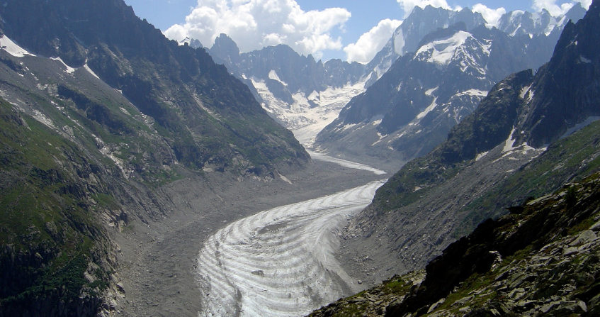
Solids can also exhibit viscous behaviour, for example when they deform over time by a phenomenon called creep. A lead wire from which a weight is suspended will gradually elongate over time by creep. More generally, different time scales or temperature variations can transform a fluid into a solid or vice versa. Thus, an ice cube will behave like a solid elastic-fragile elastic at the exit of its ice box. It is indeed a solid since it has its own shape, and, under low applied pressures, its deformations return to zero when the pressure is cancelled – its behaviour is therefore reversible and elastic. However, under a violent shock, it will break abruptly, displaying fragile behaviour. On the other hand, on a year-round basis, ice can behave like a viscous fluid: for example, the tongue of the Mer de Glace in Chamonix (Figure 2) flows at a rate of about 100 m/year following the meanders of the valley. We can deduce an estimate of its viscosity: ¹⁰¹⁶ times that of water.

An ice cube and a solid in general can break. Its clear fracture into several pieces is technically called brittle fracture, as obtained with an ice pick for ice or a hammer for glass. But there is another form of rupture, for which the material does not divide into fragments: it is the so-called ductile rupture, described by the theory of plasticity. This plastic deformation mainly corresponds to irreversible relative displacements of the components constituting the material, such as boulders, grains of sand, clay particles, grains of powders and powdery materials, metal crystals, ice crystals…

These plastic ruptures involve friction forces, internal to the materials, instantaneous and independent of speed, according to the solid friction law known as the Coulomb law (Read the focus What is the Coulomb friction law? associated with the article on sand). However, it should be remembered that, when the deformation of the solid is viscous, these internal forces increase with the deformation rate. Thus the lead wire, mentioned above, will almost instantaneously undergo elastic (reversible) elongation for a low load, plastic elongation (irreversible) for a load that exceeds the so-called failure criterion, and viscous elongation (creep) proportional to time for a lower load that remains. Iron can also undergo plastic deformations, all the more easily when its temperature is high: it thus becomes ductile. The blacksmith knows this phenomenon well, which allows him to deeply deform a metal part without breaking it into fragments. The metal flows all the better as the temperature increases, and at the melting temperature it changes state and turns into an ordinary liquid, not much more viscous than water.

In short, plastic deformations are instantaneous, while viscous deformations are delayed (spread over time). The footprint of a foot on the sand of the beach is both instantaneous and irreversible (permanent): the behaviour of the sand can therefore be described here as “plastic”. The one of a foot in a muddy field will be irreversible but will increase over time (if you freeze in place long enough!) by creep: the behaviour of the clay will be viscous here. As for the perfectly reversible deformations, which cancel each other out when the load is cancelled, we have seen that they are described by the theory of elasticity. In short, reversible deformations are elasticity; irreversible deformations are viscosity when they are a function of time; they are plasticity when they are independent of time.

Today, it is often accepted that there are no intrinsically solid materials, but rather behavioural domains with solid or fluid characteristics for a given material, whose general behaviour will be of the elasto-visco-plastic type. As an illustration, let us take the case of sand: elasto-plastic solid, on which we walk on the beach, and granular fluid, which flows into an hourglass (Figure 3).

3. Stresses and deformations

The movement of a material object assimilable to a point is entirely described by the notions of force vector and displacement vector, linked by the laws of dynamics (Read The Laws of dynamics). According to these laws, the force applied is equal to the product of the mass of this object by its acceleration. In addition, a fluid, gas or liquid, is characterized as a first approximation by its pressure and volume (if thermal aspects are not taken into account), linked by a state law.

Let us now consider a deformable solid and see why the previous notions of force-displacement or pressure-volume no longer apply and must be generalized. Let’s take the example of a bucket filled with sand. If we apply vertical pressure to it by pressing on the upper free surface, experience shows that about half of this pressure is measured on the lateral surfaces of the bucket and a little less than this pressure on the bottom of the bucket. If the bucket had been filled with water, the same pressure would have been collected everywhere: water behaves isotropically, but sand does not. It was therefore necessary to imagine a new mathematical tool to describe this pressure in a deformable solid, which varies with the direction within the solid, or more precisely with the orientation of any facet, which can be isolated by thinking within the solid and on which this pressure is applied. The notion of vector does not allow to describe this directional variation of the force per unit area. The tool that allows this description is a tensor [3] of order 2, we will see how to build it.

On each of the faces of the cube in Figure 4 is exerted a set of forces, not necessarily perpendicular to the face. The notion of pressure (always perpendicular to the surface in the case of a static fluid) must therefore be generalized by considering oblique forces with respect to the surface. The mere fact that one can walk on the ground without slipping shows that one can effectively apply tangential forces to the surface of a solid and that it can resist them. According to the principle of action and reaction, the six forces represented on the faces of the cube in Figure 4 are equal two to two on opposite faces. There are therefore only three independent force vectors. These three forces per unit area, called stress vectors, make it possible to construct a square matrix of 3 rows and 3 columns: this is the matrix of stress tensor components. It is shown that it makes it possible to calculate the surface force exerted on any facet, of any orientation, inside the material.

Thus in this case of the sand bucket, the vertical stress in the bucket will be equal to :

_σv = F / S, where F is the total vertical force applied and S is the surface of a horizontal section of the bucket. The horizontal or radial stress, applied to the side walls of the bucket, will be approximately equal to :

_σh = _σv / 2 = F / 2S.

These two constraints are called main constraints because they apply perpendicular to the respective horizontal and lateral facets.

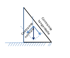
In the case of any orientation of the facet, the constrained vectors are not perpendicular to it. A distinction is then made between the stress vector projected on the plane of the facet – called shear stress or tangential stress and the one projected perpendicular to this plane, on the normal to the facet – called normal stress (see Figure 5).

Let us now return to the notion of displacement of a material point or variation in the volume of a material, which we must also generalize. Indeed, the experiment conducted on the sand bucket shows that the free upper surface of the sand settles under the action of vertical pressure exerted by the hand, while the lateral surfaces, held by the bucket, remain fixed. Here again, it appears that the displacements of these surfaces are no longer identical in all directions of space as in the case of a fluid, but on the contrary that they vary with these directions.

If we assimilate each small volume of sand to a material point, we obtain what is called a displacement field, describing the displacement of any material point of the sand – concretely, any grain of sand – in the bucket. A question arises here. In the vertical direction of the bucket, there will be significant movement near the free surface and no movement at the bottom of the bucket. They will actually vary linearly with depth. However, each small cube, subjected to the same vertical pressure, deforms itself vertically in the same way. We must therefore move from the notion of “displacement” to the more intrinsic notion of “deformation“. This is done by a gradient operation [4], which transforms the vertical displacement into a dimensionless quantity called “vertical deformation”, identical at any point of the sand and equal to the ratio of the vertical displacement of a grain of sand by the height of that grain in the bucket.

But we need to generalize this experiment, because what would happen if the walls of the bucket were to deform under the action of vertical pressure on the free surface of the sand? Then, the movement of the grains of sand would no longer be vertical but oblique. By taking the gradient of this displacement field (3-component vectors), we obtain a deformation matrix field (3 rows and 3 columns) completely characterizing the deformation of the sand in a deformable bucket.

This square matrix of 3 rows and 3 columns can actually be decomposed into the sum of two matrices: one describes the rotation of the cube of material during the application of forces and the other the actual deformation of the cube (without rotation), this is called pure deformation (see an illustration in Figure 4).

On the simple example of the rigid-walled sand bucket, the vertical deformation is equal to : _εv = δH / H, where H is the height of the bucket, while the horizontal or radial deformation is equal: _εh = δD / D, where D is the diameter of the bucket. These deformations are called main deformations because they are perpendicular to the respective horizontal and vertical or lateral surfaces.

In fact, in general, it is shown that pure deformation makes it possible to find the two fundamental modes of deformation of an elementary cube of material subjected to any kind of stress: the length of a material segment inside the cube changes and the angle between two material segments also varies during the deformation of the cube.

It was the Egyptians who first defined these two concepts of length and angle, which allowed them to recover the boundaries of their fields, covered by the silts of the Nile floods, after the passage of these floods. Even today, we still represent the deformation of matter through these two notions, and it is precisely shown that pure deformation provides us with these two quantities at any point of a deformable material.

4. Behavioural laws

Each material is deformed in a way that is unique to it and that characterizes what is called its mechanical behaviour, formalized by a mathematical relationship called the “law of behaviour“. In general, the stress at a given point in the material and at a given time is a function of the entire history of pure deformation at that point. In the case of elastic behaviour, a simple mathematical function (independent of any history) links stress to strain.

The elasticity is called linear, if this function is linear and a proportionality relationship then links stresses and deformations: the stress matrix is, in this case, equal to the elastic tensor multiplied by the deformation matrix. In the usual case of isotropic elastic material (its behaviour is identical in all directions of space), this tensor depends on only two parameters: Young’s modulus (characterizing the stiffness of the material) and the fish coefficient (reflecting its ability to deform laterally under axial compression).

Newtonian viscosity, the simplest of the viscous laws, translates into a proportionality relationship between stress and pure deformation rate at the same time. This type of relationship thus makes it possible to describe the increase in the strength of the material with the speed of application of the forces.

Finally, in elasto-plasticity, this relationship between stress and strain is no longer univocal as in pure elasticity and we then prefer to use a so-called incremental writing linking a small variation in stress to a small variation in strain. An elasto-plastic tensor is thus created, connecting the incremental stress to the incremental deformation in a proportional way. The material that most faithfully obeys an elasto-plastic behaviour is sand. Thus, a sand pile or a balanced dune has a slope (Figure 6), the angle (around 30°) of which corresponds to the internal plastic friction between the grains of sand. On the contrary, a viscous liquid, devoid of plasticity, would gradually spread out over time. The plastic behaviour of the sand allows the slope to be stable without spreading. However, if a little sand is added along the slope, a local avalanche occurs immediately, showing that the mechanical state of the sand here corresponds to a state of plasticity called “limit” corresponding to the failure criterion mentioned in section 2: this slope limit angle cannot be exceeded.

One of the interesting properties of plasticity is the phenomenon of strain hardening, which reflects the possibility of improving the mechanical strength of a material by plastically deforming it. A remarkable illustration is the implementation of the underlay of a pavement. The sand is dumped by trucks and its very loose condition allows it only a very low resistance: a finger can sink into it. But, once compacted by rollers that strain it very hard, the sand layer becomes remarkably resistant: a car can already drive on this layer. However, if there is no glue between the sand grains, it will have difficulty braking because the sand grains will not provide sufficient resistance to tire slippage. Bitumen provides this glue: it ensures the cohesion of the sand or its mixture with gravel. But, on the other hand, this cohesion creates the possibility of cracks, which degrade the pavement..

We understand here the intrinsic numerical difficulties involved in the calculation of a metal structure, the sizing of a civil engineering structure, the prediction of the flow of a complex fluid or, more generally, the behaviour of any mechanical system, since it is true that the elasto-visco-plastic behaviour of materials is complex to calibrate experimentally and to describe numerically. But how can we precisely calculate – that is, ultimately predict – the mechanical behaviour of a system subjected to forces that can change over time?

5. Solving a problem in the mechanics of deformable materials

Whether considering fluids or solids, to calculate and predict the behaviour of a structure and a structure, the engineer has to write and solve three groups of mathematical equations of a very different nature:

• Conservation laws (of mass, energy, amount of movement, etc.), valid regardless of the material and the problem considered. These laws have generally been known and formalised for a very long time.
• The laws of behaviour of materials whose formalization we have described in this article. These laws, which are, in the most general case, elasto-visco-plasticity as we have seen, are still the subject of active research and nowadays incorporate a detailed description of the microstructure of materials (and even of their nano-structure, when we consider nano-materials today).
• The initial and boundary conditions that define the system, mechanical structure, structure, structure, flow, etc., that are being modelled. The initial conditions characterize the initial state (at the beginning of the calculation) of the system. Boundary conditions, on the other hand, determine all the geometries and forces that will be applied over time. Industrial calculation codes are currently able to take into account a very wide variety of such conditions.

Sometimes several physicochemical phases are present (for example, soil, air and water, or rock, oil and gas) and we speak of multi-phase environments. In other cases, the problem reveals “coupled” loads. These are called multi-physical problems (for example, coupling between mechanics and thermics if the temperature occurs, or coupling between mechanics and chemistry in the case of chemical reactions between the components of the system, etc.).

For the engineer, the most delicate question most often lies in the choice and implementation of behavioural laws, as representative as possible of the materials concerned in the problem under consideration. Modern numerical methods make it possible to solve the system of equations formed by the three groups of equations mentioned above. The number of equations can reach several million and requires the use of supercomputers.

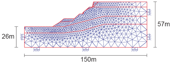
While it can be assumed that the continuity of the material is respected during its deformation, the best known method is the so-called “finite element” method (Figures 7 and 8). The calculation presented on these two figures made it possible to digitally model, and therefore understand, a landslide that actually occurred in Trevoux after torrential rains (see Landslides).

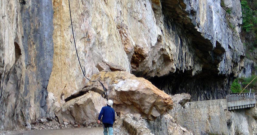
Today we could quantify critical rainfall. Prevention devices (walls, embankments, soil reinforcement, drainage, etc.) can also be digitally tested to validate or not their effectiveness. On the other hand, if the materials have intrinsic and irreducible discontinuities (for example, in the case of fracturing the material such as a fractured cliff), another numerical method called “discrete elements” can be used (Figure 9). We then obtain by numerical calculation the displacements and rotations of each elementary block, which can number several million. For example, the fragmentation of a concrete block impacted by a projectile can be simulated numerically. This method also allows the calculation of avalanches (of snow, boulders,…) and torrential mudflows. (Read Landslides and rockfalls, a fatality?).

 

---

References and notes

Cover image. The Millau cable-stayed bridge is an example of a structure whose design has required in-depth studies on the behaviour of its constituent materials. Source: Wikipedia, Attribution License – Sharing of the identical initial conditions v. 2.5 of Creative Commons, better known as “CC-BY-SA-2.5; © Mike Lehmann, Mike Switzerland 10:38, 14 March 2008 (UTC)”.

[1] Rheology is the science that describes how matter flows or, more generally, is distorted. The word comes from the Greek “ρεω” which means “to flow” and from “λοϒοσ” “speech”.

[2] In the case of vehicles or other large objects, the driving resistance is dominated by turbulence and viscosity has little influence.

[3] A tensor is a mathematical object that respects the so-called rules of tensoriality. These rules allow us to continue to describe the same physical being, whatever the benchmark we have chosen to express its components. The components of a first-order tensor, which is a vector, form a row or column of numbers; those of a second-order tensor form a matrix (table of numbers). Stresses and deformations are thus represented using matrices. Tensors of any finite order are defined. For example, the elastic tensor (discussed below) is of order 4.

[4] The gradient of a scalar function is a vector whose components are the partial derivatives of the function with respect to spatial coordinates. By extension, the gradient of a vector is a matrix whose column vectors are made up of partial derivatives of each of the vector’s components with respect to spatial coordinates. In the classic 3-dimensional space, this results in a square matrix of 3 rows and 3 columns.