Climate variability: the example of the North Atlantic Oscillation

Will there be snow this winter? Should we go on holiday in Brittany or on the French Riviera? Will the harvest be good this year? All these questions clearly show the whims of the seasons, especially at our latitudes. It has long been known that these fluctuations are partly organized, but it is still difficult to predict them.

1. What is climate variability?

Climate is traditionally defined by the average, over about 30 years, of locally measured meteorological parameters: pressure, temperature, wind, precipitation, cloud cover, etc. These climatological averages are often referred to as “normal“: they are referred to as “seasonal normals” as the expected values for the season. First, they depend on the supply of solar energy, as the etymology of the Greek word ‘climate’ reminds us: ‘inclination of the sky’, i.e. the rays of the Sun. But in reality, weather conditions are always a little different from their average. These fluctuations constitute climate variability, and are as important for characterizing climate as their average, for several reasons.

First of all, their amplitude is a characteristic of the climate itself: overall, this variability increases with latitude, so it is low in the equatorial region and high in the polar regions.

In addition, their impacts on ecosystems and societies are much greater than regular seasonal variations: a cool, humid summer or a dry, snow-free winter, for example, have consequences on vegetation, agriculture and economic activities. Heat waves, cold waves, storms… if extreme fluctuations remain rare, their impacts are even stronger, sometimes catastrophic. Recently, the European Environment Agency estimated the cost of climate-related disasters in Europe at €12 billion per year [1].

Finally, these fluctuations are partly organized, in time and space: these preferential organizations are called “modes of variability“. They have a certain persistence over time, which makes it possible to consider their prediction. This article discusses a mode of variability.

At mid-latitudes, the atmospheric circulation is essentially’horizontal’ (see Atmospheric circulation: its organization). The confrontation of warm air from low latitudes and cold air from high latitudes produces disturbances of several thousand kilometres. Transported by general traffic, they cause weather fluctuations (Section 2). These fluctuations are partly organized, on time scales ranging from week to decade, according to several organizational modes. In the North Atlantic, one mode is particularly pronounced: the “North Atlantic Oscillation“, known as NAO, which stands for “North Atlantic Oscillation” (Section 3). This regional mode is part of an even broader mode that dominates the variability of the entire northern hemisphere, called “Arctic Oscillation” or also “Northern Hemisphere Annular Mode” (Section 4).

2. Medium latitudes: “synoptic” fluctuations

2.1. A zonal circulation of the atmosphere

At mid-latitudes the general atmospheric circulation is called “zonal”: it is from west to east, and it is structured by high altitude “jet” currents (see Atmospheric circulation: its organization and Jet streams).

In the lower atmosphere, westerly winds are wavering between areas of low and high pressure. Regularly, low pressure centres are’deepening’ (their pressure decreases) over the Atlantic to form cyclonic disturbances. The latter bring disturbed and rainy weather to the west coast of Europe, with weather conditions changing in a few days and affecting a region over a thousand kilometres. Between these disturbances, areas of high anticyclonic pressures induce calm and stable weather.

Sometimes, these high pressures “park” on a region, and divert the disturbances: we speak then of “blockage” of the zonal traffic. Passage of disturbances, anticyclonic conditions, even persistent blocking conditions… all phenomena that cause meteorological fluctuations in Western Europe, referred to as “synoptic variability“.

2. How are weather conditions measured?

This circulation and its disturbances are directly related to differences in atmospheric pressure. The barometer does nothing more than announce rain when the pressure drops, or a great sunny day when it rises. For forecasting purposes, the first networks of meteorological stations were set up in Europe at the end of the 18th century by various institutions: the Royal Society of Medicine in France, the Palatine Society of Mannheim (now Germany), later in 1854 the Royal Meteorological Service in England [2]. These networks are now managed by each country and coordinated by the World Meteorological Organization (WMO). This provides a long series of measurements of weather conditions in Europe.

Upper air measurements were then made by balloon and then by satellite over the past 30 years. These measurements and observations are sent and compiled several times a day to WMO. They are used for weather forecasting by the assimilation technique (see Introduction to weather forecasting and Assimilation of meterological data). Past measurements are also assimilated by atmospheric circulation models. Objective: Simulate past weather conditions, including unmeasured regions and altitudes. Called “reanalyses“, these simulations are interpolations of scattered data to obtain a global and physically coherent view of the state of the atmosphere. These re-analyses are widely used by climatologists to study and characterize climate and its variability. They currently date back to the beginning of the 20th century, and to the 19th century on an experimental basis.

On the oceans, measurements are much more recent and remained very scattered before the advent of satellites. Here too, considerable work is being done to obtain reliable temperature series and to study their variability: the aim is to compile, correct and homogenize water temperature measurements made by boats. From the 1960s onwards, vertical ocean temperature profiles began to be developed systematically. Since the 2000s, a network of autonomous floats has been used to regularly probe the first two kilometres of the ocean. In general, ocean temperature varies much less spatially and temporally than on continents: this lower variability makes it possible to obtain a correct reconstruction of the ocean surface with far fewer measurements.

3. The North Atlantic Oscillation, an organization of weather conditions

3.1. A shift of air masses

18th century notes [3] report that winter conditions were often in opposition between Denmark and its trading posts in West Greenland, between wet mildness and dry cold. Past accounts also mention links between weather conditions in different parts of the world. These empirical observations were then explored using a series of measurements. These studies [4] have shown strong statistical relationships between various meteorological parameters over several thousand kilometres: these remote links are called “teleconnections” (etymologically “remote links”). These teleconnections reveal a preferential organization of atmospheric circulation and associated meteorological conditions, which is called a mode of variability.

It should be remembered that a statistical correlation is a close relationship between two parameters that vary jointly (in the same direction). If these two parameters vary in opposite directions, it is an anti-correlation. Figure 1 illustrates one of the teleconnections related to the North Atlantic Oscillation, between the Icelandic Low and the Azores High. This is the very “engine” of this oscillation: a set of air masses, and therefore atmospheric pressure, shifting between the south and north of the North Atlantic basin. It is this pressure shift that climatologists have referred to as seesaw.

3.2. The NAO index of this oscillation

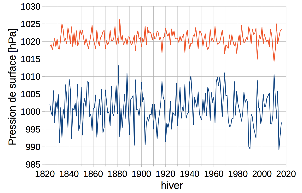
Over the course of the studies [5], this pressure shift between south and north of the North Atlantic basin has emerged as the most important feature of this NAO mode. On the one hand, this shift induces a strong teleconnection between these two regions (Figure 1), and on the other hand it is able to modify the trajectory of the disturbances that cross the Atlantic. An index of the activity of this Oscillation – the NAO index – was therefore established from the pressure measurements (Figure 1). NAO activity is strong when there is a strong pressure shift between Iceland and the Azores (regions called’action centres‘). A strong shift implies large fluctuations in pressure around its average in each of these centres, and that these fluctuations are opposite (anti-correlated). In contrast, NAO activity is low when the pressure does not vary jointly in the south and north, or when the pressure varies little. The NAO index is calculated to oscillate around zero. Thus, it is positive when the scale tilts north, negative when it tilts south, and close to zero when the scale is flat (low NAO activity). The higher its value, the more the pressure switch is tilted.

In practice, several techniques are used to calculate indices that are quite similar (Figure 2). The simplest index is based on pressure measurements taken at a few stations in Iceland and southwest Europe (Azores and/or Iberian Peninsula). This index, in blue in Figure 2, thus makes it possible to trace the NAO activity back to the 1820s. Another technique uses the pressure fields covering the entire Atlantic region, resulting from the reanalyses. A corresponding index is in red in Figure 2: it is more accurate, but does not go back that far in time.

3.3. A ten-year persistence of this NAO mode

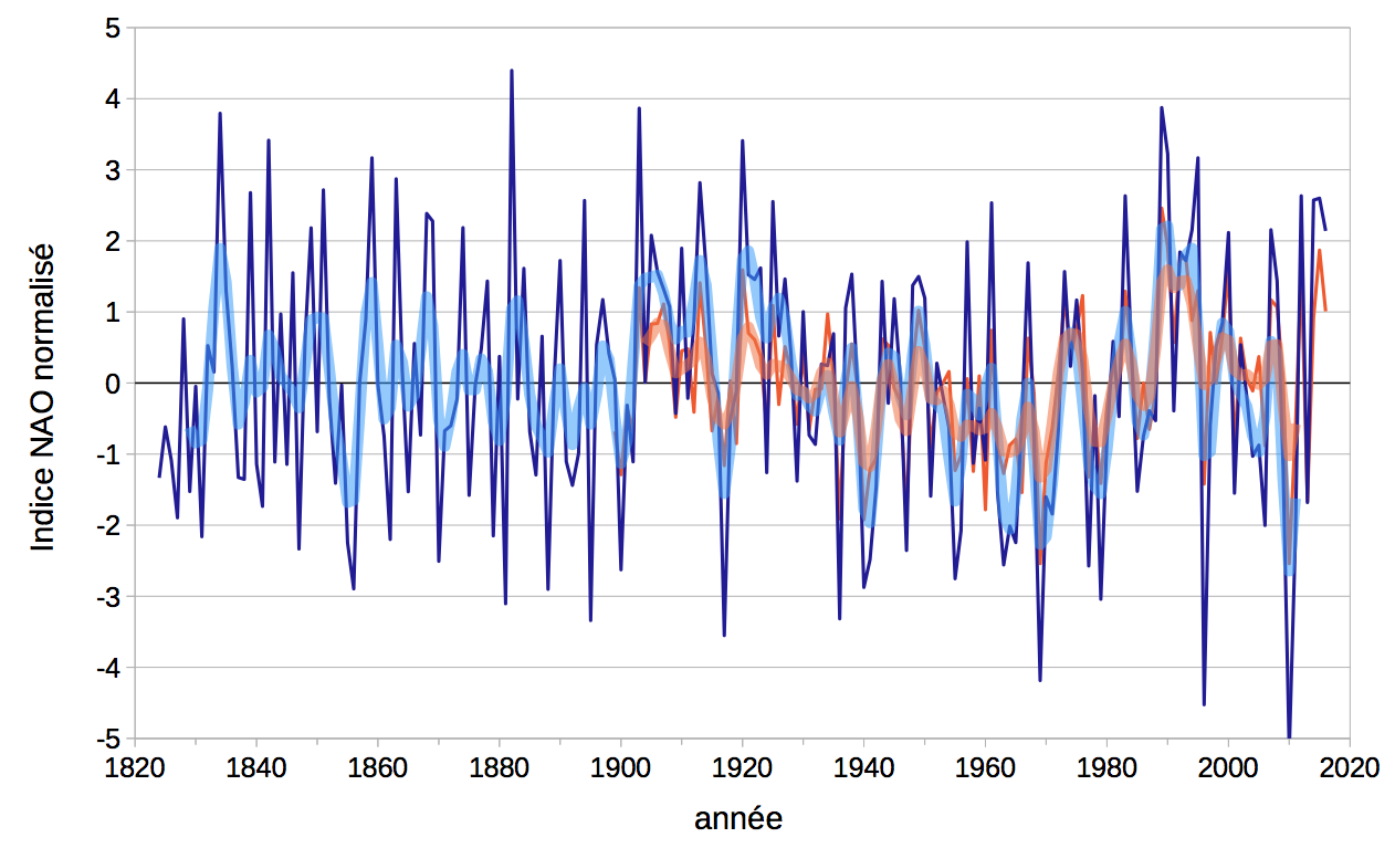
Figure 2 shows that this pressure shift between north and south of the North Atlantic varies greatly from one winter to the next (referred to as the inter-annual scale), but it shows some persistence over 10 to 20 years (10-year scale). In particular, the decades 1900-1910, 1920-1930, and 1990-2000 were marked by a positive phase of the changeover (called “NAO+”) with a fairly positive average index. In contrast, the decades 1850-1860 and 1950-1970 were marked by a negative phase (‘NAO-‘). But such persistence does not prevent extreme values in the opposite direction: the winter of 1995-96, for example, was marked by a particularly negative index value in the middle of a rather positive decade.

3.4. What are the impacts on weather conditions?

As mentioned above, the pressure shift between north and south of the North Atlantic region mainly modifies the trajectory of disturbances crossing the North Atlantic at mid-latitudes, but also the westerly wind speeds associated with these trajectories. The impact of this shift on weather conditions is therefore opposite between north and south of Western Europe. In summer, more frequent disturbances lead to wetter and cooler conditions. In winter, the associated conditions are more humid and mild, typically rain instead of dry cold in northern Europe.

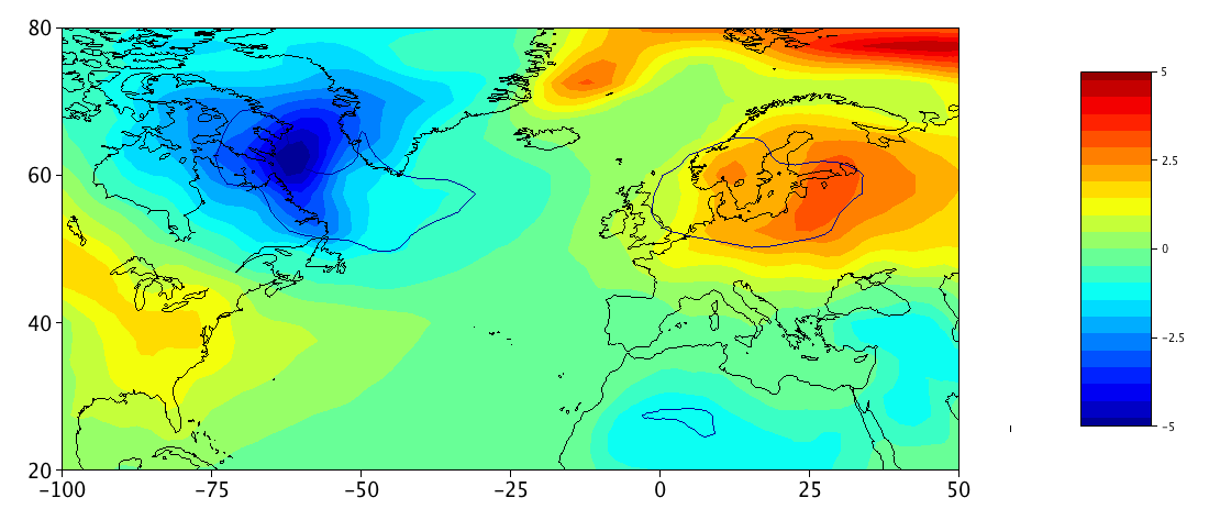
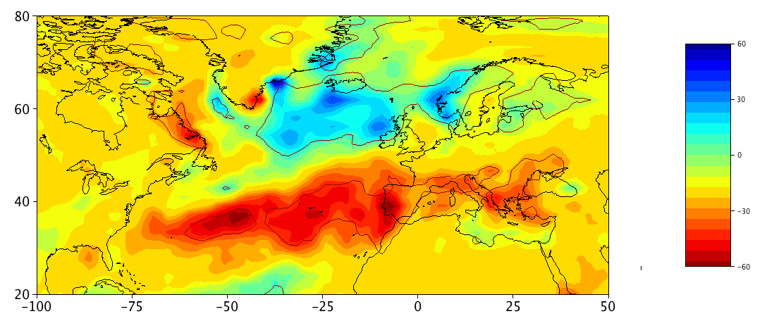
Figure 3 illustrates the typical meteorological impacts of the North Atlantic Oscillation for the month of January. These impacts are not restricted to Western Europe: they also affect the eastern edge of North America, due to the circulation changes induced by the north-south pressure shift. A very strong teleconnection exists in temperature between the Labrador region and Scandinavia, and in a more moderate way between the east coast of the United States and the Mediterranean and North Africa (as far as the Near East). It can be noted that the temperature of the action centres is not affected, whereas these centres are the drivers of weather fluctuations. Precipitation anomalies have a more “zonal” spatial structure, with a north-south contrast similar to the pressure shift, and extremes close to the action centres.

However, these impacts are relatively small compared to winter-to-winter fluctuations (inter-annual variability), especially for precipitation. The colored contours in Figure 3 define the regions for which these impacts are marked. At most, the NAO mode thus only describes 20 to 30% of the inter-annual temperature variability.

But have these meteorological impacts of the North Atlantic Oscillation affected the European climate? One of the best recent examples is the marked transition from the rather negative NAO conditions of the 1960s to 1980s, to the rather positive in the early 1990s. This transition is responsible for the warming of Western Europe, which is faster and more significant than that of the rest of the world and than predicted by climate models [6]. One of the most visible consequences of this warming was a decrease in snowfall in the Western Alps [7]. This positive NAO phase lasted about a decade, then the Oscillation turned into a negative phase on average, with sometimes very negative indices (historical low of winter 2009-2010). This period of negative phase was accompanied by remarkable winter cold spells (December 2001) and fairly cold winters on average (2004-05, 2005-06, 2009-10, 2010-11). However, apart from these few cold winters, the other winters of the 2000 and 2010 decades were rather hot or even very hot in France. It therefore seems that the North Atlantic Oscillation has less impact on weather conditions. Various studies have simulated weather conditions in Europe taking into account traffic (including NAO phases): they show that, since the late 1990s, actual weather conditions have been warmer than expected, including in the cold winters of the 2000s [8].

4. Other regional ways of organizing the atmosphere

In the 19th and 20th centuries, meteorologists compared all available series of measurements to find correlations between regions. The North Atlantic basin was very quickly recognized as a region with strong teleconnections, due to the North Atlantic Oscillation. But ways of organizing the atmosphere have emerged in other regions. This is the case of the famous Southern Oscillation (SO) in the tropical Pacific. It was by studying the Indian monsoon, a phenomenon of considerable importance for India, that Gilbert Walker highlighted the Southern Oscillation at the beginning of the 20th century. This oscillation is associated with the powerful ENSO phenomenon (see ENSO article – in preparation).

From the 1980s onwards, the technique of data assimilation by atmospheric models made it possible to make considerable progress (see Assimilation of meteorological data). The analyses from these models provided a global view of atmospheric circulation and its variability. They also made it possible to explore its organization much further, with different statistical tools (e. g. main component analyses). Modes affecting an entire hemisphere have thus been identified at mid- and high latitudes. The organization of these modes is called “annular” with a pressure shift between the polar zone and the surrounding mid-latitudes (ring structure). These are the Northern annular mode (NAM), more commonly known as Arctic Oscillation (AO), and the Southern annular mode (SAM).

In the annular mode of the northern hemisphere, the Atlantic region plays a major role, with a very high variability in atmospheric circulation, but also a very marked organization. Moreover, this region does not always play the same score as the other regions of the northern hemisphere. For these reasons, the North Atlantic Oscillation clearly stands out as a particular regional mode.

Generally, these modes describe the organization of atmospheric circulation on time scales that range from week (synoptic) to season. The North Atlantic Oscillation also shows some persistence over several years, which is very long in relation to the rate of change in the atmosphere. To try to explain such persistence, climatologists looked to the oceans. Indeed, their surface has a much higher thermal inertia than that of the atmosphere (we speak of the ocean as a “thermal flywheel”); the speed of ocean currents is also much lower than that of winds. This planet’s thermal flywheel was therefore an ideal candidate to explain the ten-year persistence of certain modes such as NAO.

The study of ocean surface temperature has thus led to the identification of several ocean-specific modes. In the northern hemisphere, it is the Atlantic multi-decadal oscillation (AMO), which describes the temperature anomaly of the North Atlantic basin, and the Pacific decadal oscillation (PDO), which describes a temperature shift between the eastern and western areas of the North Pacific. The tropical zone is dominated by the ‘El Niño / la Niña’ mode, a component of the ENSO mode describing the shift of a temperature anomaly between the east and west of the equatorial Pacific (see ENSO article – in preparation).

In fact, this idea of the ocean’s “flywheel” to explain the ten-year persistence of NAO phases has proved more complicated than expected. Indeed, theoretical studies [9] show that synoptic fluctuations in atmospheric circulation (of the order of a week) are filtered by the surface ocean to create ocean temperature and/or circulation anomalies of several years. Some studies suggest that the North Atlantic Oscillation, which affects the atmosphere, is responsible for the multi-decadal Oscillation of the Atlantic Ocean. In the opposite direction to what was expected! The positive NAO phase of the 1990s would thus be at the origin of the warming of the North Atlantic Ocean since the mid-1990s, corresponding to the transition from the multi-decadal Atlantic Oscillation to a positive phase. This warm Atlantic anomaly may be responsible for the warm conditions of the 2010 decade in Europe.

5. Conclusion: Origin of the NAO and forecasting potential

After a century of research on the North Atlantic Oscillation, what is the outcome? First of all, it is a privileged organization of atmospheric circulation in the North Atlantic basin, with two opposite phases (NAO+ vs. NAO-), particularly marked in winter. This organization is quite well reproduced by digital models of the atmosphere. However, the factors of this organization, the sometimes abrupt transition between these two phases, and the ten-year persistence of a phase have not yet been clearly identified. On a weekly scale, the tropical zone seems to be responsible for the phase change via the propagation of wave trains in the atmosphere. At the scale of the season, especially in winter, taking into account the surface state of the high latitudes and the upper atmosphere seems to give the best forecasts of the NAO phase. On the other hand, persistence on a ten-year scale remains difficult to explain, even if the ocean’s “inertial flywheel” remains a good candidate.

In the end, the North Atlantic region is probably one of the regions most scrutinized by meteorologists and climatologists, with the longest series of measurements. But it is also a region under very strong influences, from the tropics, the Arctic, the eastern Pacific, and even the stratosphere. Predicting the seasonal evolution of atmospheric circulation, even if only that of the North Atlantic Oscillation, has remained a challenge for more than 50 years [10]. Even though the societal impacts are very strong in this region.

---

References and notes

Cover image. Pixabay.

[1] Indicator:Economic losses from climate-related extremes, accessed on 17/02/2017.

[2] This service was led by the famous Robert FitzRoy, explorer and captain of the HMS Beagle with Darwin.

[3] Stories by missionary Saabye of the contrasting conditions between Greenland and Denmark during the period 1770-78, cited by van Loon & Rogers (1978), Monthly Weather Review, 106, 296-310

[4] Teisserenc de Bort (1883) Study on the winter of 1879-80 and research on the influence of the position of the major centres of atmospheric action in abnormal winters. Annales de la Société Météorologique de France, 31, 70-79; Hildebrandsson & Teisserenc De Bort (1907) Les bases de la météorologie dynamique, Gauthier-Villars, Paris.

[5] Walker & Bliss (1932). World weather V, Mem Royal Meteorol Soc, 4(36), 53-84.

[6] van Oldenborgh et al. (2009). Western Europe is warming much faster than expected. Climate of the Past 5: 1-12, DOI: 10.5194/cp-5-1-2009. Delworth et al. (2016) The North Atlantic Oscillation as a driver of rapid climate change in the Northern Hemisphere. Nature Geoscience 9: 509-512, DOI:10.1038/ngeo2738

[7] Beniston (2012). Is snow in the Alps receding or disappearing? WIRes 3: 349-358, DOI: 10.1002/wcc.179

[8] Yiou et al. (2007). Inconsistency between atmospheric dynamics and temperatures during the exceptional 2006/2007 fall/winter and recent warming in Europe. Geophys Res Lett 34:L21808. DOI: 10.1029/2007GL031981

[9] Frankignoul & Hasselmann (1977). Stochastic Climate Models 2 Application to Sea-Surface Temperature Anomalies and Thermocline Variability. Tellus, 29, 289-305.

[10] Woollings (2010). Dynamical influences on European climate: an uncertain future. Philosophical Transactions of the Royal Society of London 368: 3733-3756, DOI:10.1098/rsta.2010.0040