Climate variability: the example of the North Atlantic Oscillation

PDF
variabilité climatique - climat - vague froid - vague froid exceptionnel - hiver - neige - encyclopedie environnement - north atlantic oscillation

Will there be snow this winter? Should we go on holiday in Brittany or on the French Riviera? Will the harvest be good this year? All these questions clearly show the whims of the seasons, especially at our latitudes. It has long been known that these fluctuations are partly organized, but it is still difficult to predict them.

1. What is climate variability?

Climate is traditionally defined by the average, over about 30 years, of locally measured meteorological parameters: pressure, temperature, wind, precipitation, cloud cover, etc. These climatological averages are often referred to as “normal“: they are referred to as “seasonal normals” as the expected values for the season. First, they depend on the supply of solar energy, as the etymology of the Greek word ‘climate’ reminds us: ‘inclination of the sky’, i.e. the rays of the Sun. But in reality, weather conditions are always a little different from their average. These fluctuations constitute climate variability, and are as important for characterizing climate as their average, for several reasons.

First of all, their amplitude is a characteristic of the climate itself: overall, this variability increases with latitude, so it is low in the equatorial region and high in the polar regions.

In addition, their impacts on ecosystems and societies are much greater than regular seasonal variations: a cool, humid summer or a dry, snow-free winter, for example, have consequences on vegetation, agriculture and economic activities. Heat waves, cold waves, storms… if extreme fluctuations remain rare, their impacts are even stronger, sometimes catastrophic. Recently, the European Environment Agency estimated the cost of climate-related disasters in Europe at €12 billion per year [1].

Finally, these fluctuations are partly organized, in time and space: these preferential organizations are called “modes of variability“. They have a certain persistence over time, which makes it possible to consider their prediction. This article discusses a mode of variability.

At mid-latitudes, the atmospheric circulation is essentially’horizontal’ (see Atmospheric circulation: its organization). The confrontation of warm air from low latitudes and cold air from high latitudes produces disturbances of several thousand kilometres. Transported by general traffic, they cause weather fluctuations (Section 2). These fluctuations are partly organized, on time scales ranging from week to decade, according to several organizational modes. In the North Atlantic, one mode is particularly pronounced: the “North Atlantic Oscillation“, known as NAO, which stands for “North Atlantic Oscillation” (Section 3). This regional mode is part of an even broader mode that dominates the variability of the entire northern hemisphere, called “Arctic Oscillation” or also “Northern Hemisphere Annular Mode” (Section 4).

2. Medium latitudes: “synoptic” fluctuations

2.1. A zonal circulation of the atmosphere

At mid-latitudes the general atmospheric circulation is called “zonal”: it is from west to east, and it is structured by high altitude “jet” currents (see Atmospheric circulation: its organization and Jet streams).

In the lower atmosphere, westerly winds are wavering between areas of low and high pressure. Regularly, low pressure centres are’deepening’ (their pressure decreases) over the Atlantic to form cyclonic disturbances. The latter bring disturbed and rainy weather to the west coast of Europe, with weather conditions changing in a few days and affecting a region over a thousand kilometres. Between these disturbances, areas of high anticyclonic pressures induce calm and stable weather.

Sometimes, these high pressures “park” on a region, and divert the disturbances: we speak then of “blockage” of the zonal traffic. Passage of disturbances, anticyclonic conditions, even persistent blocking conditions… all phenomena that cause meteorological fluctuations in Western Europe, referred to as “synoptic variability“.

2. How are weather conditions measured?

This circulation and its disturbances are directly related to differences in atmospheric pressure. The barometer does nothing more than announce rain when the pressure drops, or a great sunny day when it rises. For forecasting purposes, the first networks of meteorological stations were set up in Europe at the end of the 18th century by various institutions: the Royal Society of Medicine in France, the Palatine Society of Mannheim (now Germany), later in 1854 the Royal Meteorological Service in England [2]. These networks are now managed by each country and coordinated by the World Meteorological Organization (WMO). This provides a long series of measurements of weather conditions in Europe.

Upper air measurements were then made by balloon and then by satellite over the past 30 years. These measurements and observations are sent and compiled several times a day to WMO. They are used for weather forecasting by the assimilation technique (see Introduction to weather forecasting and Assimilation of meterological data). Past measurements are also assimilated by atmospheric circulation models. Objective: Simulate past weather conditions, including unmeasured regions and altitudes. Called “reanalyses“, these simulations are interpolations of scattered data to obtain a global and physically coherent view of the state of the atmosphere. These re-analyses are widely used by climatologists to study and characterize climate and its variability. They currently date back to the beginning of the 20th century, and to the 19th century on an experimental basis.

On the oceans, measurements are much more recent and remained very scattered before the advent of satellites. Here too, considerable work is being done to obtain reliable temperature series and to study their variability: the aim is to compile, correct and homogenize water temperature measurements made by boats. From the 1960s onwards, vertical ocean temperature profiles began to be developed systematically. Since the 2000s, a network of autonomous floats has been used to regularly probe the first two kilometres of the ocean. In general, ocean temperature varies much less spatially and temporally than on continents: this lower variability makes it possible to obtain a correct reconstruction of the ocean surface with far fewer measurements.

3. The North Atlantic Oscillation, an organization of weather conditions

3.1. A shift of air masses

18th century notes [3] report that winter conditions were often in opposition between Denmark and its trading posts in West Greenland, between wet mildness and dry cold. Past accounts also mention links between weather conditions in different parts of the world. These empirical observations were then explored using a series of measurements. These studies [4] have shown strong statistical relationships between various meteorological parameters over several thousand kilometres: these remote links are called “teleconnections” (etymologically “remote links”). These teleconnections reveal a preferential organization of atmospheric circulation and associated meteorological conditions, which is called a mode of variability.

It should be remembered that a statistical correlation is a close relationship between two parameters that vary jointly (in the same direction). If these two parameters vary in opposite directions, it is an anti-correlation. Figure 1 illustrates one of the teleconnections related to the North Atlantic Oscillation, between the Icelandic Low and the Azores High. This is the very “engine” of this oscillation: a set of air masses, and therefore atmospheric pressure, shifting between the south and north of the North Atlantic basin. It is this pressure shift that climatologists have referred to as seesaw.

3.2. The NAO index of this oscillation

pression atmospherique - islance - açores - climat - hiver - schema - encyclopedie environnement - winter averages of ground atmospheric pressure
Figure 1. Winter averages of ground atmospheric pressure measured in Iceland (in blue) and the Azores (in red), in hundreds of Pascals (hPa). There is an average difference of around 20 hPa between the’Icelandic depression’ and the’Azores high’. It is also noted that for many winters, while the pressure is well above average for one region, it is below average for the other region, and vice versa (anticorrelation). The correlation coefficient is -0.6. [© G. Delaygue]

Over the course of the studies [5], this pressure shift between south and north of the North Atlantic basin has emerged as the most important feature of this NAO mode. On the one hand, this shift induces a strong teleconnection between these two regions (Figure 1), and on the other hand it is able to modify the trajectory of the disturbances that cross the Atlantic. An index of the activity of this Oscillation – the NAO index – was therefore established from the pressure measurements (Figure 1). NAO activity is strong when there is a strong pressure shift between Iceland and the Azores (regions called’action centres‘). A strong shift implies large fluctuations in pressure around its average in each of these centres, and that these fluctuations are opposite (anti-correlated). In contrast, NAO activity is low when the pressure does not vary jointly in the south and north, or when the pressure varies little. The NAO index is calculated to oscillate around zero. Thus, it is positive when the scale tilts north, negative when it tilts south, and close to zero when the scale is flat (low NAO activity). The higher its value, the more the pressure switch is tilted.

In practice, several techniques are used to calculate indices that are quite similar (Figure 2). The simplest index is based on pressure measurements taken at a few stations in Iceland and southwest Europe (Azores and/or Iberian Peninsula). This index, in blue in Figure 2, thus makes it possible to trace the NAO activity back to the 1820s. Another technique uses the pressure fields covering the entire Atlantic region, resulting from the reanalyses. A corresponding index is in red in Figure 2: it is more accurate, but does not go back that far in time.

3.3. A ten-year persistence of this NAO mode

climat - indices - oscillation nord atlantique - hiver - pression surface - schema - encyclopedie environnement - north atlantic oscillation
Figure 2. Two indices of the North Atlantic Oscillation in winter, based on surface pressure. In blue: difference between the normalized pressures measured in Gibraltar and Iceland (CRU/UEA data). In orange: first main component of the NCEP surface pressure analysis (data J. Hurrell/NCAR). Bold curves: sliding averages over 11 seasons. [© G. Delaygue]

Figure 2 shows that this pressure shift between north and south of the North Atlantic varies greatly from one winter to the next (referred to as the inter-annual scale), but it shows some persistence over 10 to 20 years (10-year scale). In particular, the decades 1900-1910, 1920-1930, and 1990-2000 were marked by a positive phase of the changeover (called “NAO+”) with a fairly positive average index. In contrast, the decades 1850-1860 and 1950-1970 were marked by a negative phase (‘NAO-‘). But such persistence does not prevent extreme values in the opposite direction: the winter of 1995-96, for example, was marked by a particularly negative index value in the middle of a rather positive decade.

3.4. What are the impacts on weather conditions?

As mentioned above, the pressure shift between north and south of the North Atlantic region mainly modifies the trajectory of disturbances crossing the North Atlantic at mid-latitudes, but also the westerly wind speeds associated with these trajectories. The impact of this shift on weather conditions is therefore opposite between north and south of Western Europe. In summer, more frequent disturbances lead to wetter and cooler conditions. In winter, the associated conditions are more humid and mild, typically rain instead of dry cold in northern Europe.

climat - indices - oscillation nord atlantique - hiver - pression surface - schema - encyclopedie environnement

climat - NAO - temperature - precipitation - schema - encyclopedie environnement - average impacts of NOA -
Figure 3. Average impacts of NAO+ conditions for the month of January (monthly averages with NAO indices. Above: temperature anomaly in ºC. Bottom: precipitation anomaly in mm/month. The colored contours give an idea of the regions for which these anomalies are significant in relation to the interannual variability (standard deviation anomaly ratio of 0.8, top, and 0.5, bottom). NCEP re-analyses 1948-2010. [© G. Delaygue]

Figure 3 illustrates the typical meteorological impacts of the North Atlantic Oscillation for the month of January. These impacts are not restricted to Western Europe: they also affect the eastern edge of North America, due to the circulation changes induced by the north-south pressure shift. A very strong teleconnection exists in temperature between the Labrador region and Scandinavia, and in a more moderate way between the east coast of the United States and the Mediterranean and North Africa (as far as the Near East). It can be noted that the temperature of the action centres is not affected, whereas these centres are the drivers of weather fluctuations. Precipitation anomalies have a more “zonal” spatial structure, with a north-south contrast similar to the pressure shift, and extremes close to the action centres.

However, these impacts are relatively small compared to winter-to-winter fluctuations (inter-annual variability), especially for precipitation. The colored contours in Figure 3 define the regions for which these impacts are marked. At most, the NAO mode thus only describes 20 to 30% of the inter-annual temperature variability.

But have these meteorological impacts of the North Atlantic Oscillation affected the European climate? One of the best recent examples is the marked transition from the rather negative NAO conditions of the 1960s to 1980s, to the rather positive in the early 1990s. This transition is responsible for the warming of Western Europe, which is faster and more significant than that of the rest of the world and than predicted by climate models [6]. One of the most visible consequences of this warming was a decrease in snowfall in the Western Alps [7]. This positive NAO phase lasted about a decade, then the Oscillation turned into a negative phase on average, with sometimes very negative indices (historical low of winter 2009-2010). This period of negative phase was accompanied by remarkable winter cold spells (December 2001) and fairly cold winters on average (2004-05, 2005-06, 2009-10, 2010-11). However, apart from these few cold winters, the other winters of the 2000 and 2010 decades were rather hot or even very hot in France. It therefore seems that the North Atlantic Oscillation has less impact on weather conditions. Various studies have simulated weather conditions in Europe taking into account traffic (including NAO phases): they show that, since the late 1990s, actual weather conditions have been warmer than expected, including in the cold winters of the 2000s [8].

4. Other regional ways of organizing the atmosphere

In the 19th and 20th centuries, meteorologists compared all available series of measurements to find correlations between regions. The North Atlantic basin was very quickly recognized as a region with strong teleconnections, due to the North Atlantic Oscillation. But ways of organizing the atmosphere have emerged in other regions. This is the case of the famous Southern Oscillation (SO) in the tropical Pacific. It was by studying the Indian monsoon, a phenomenon of considerable importance for India, that Gilbert Walker highlighted the Southern Oscillation at the beginning of the 20th century. This oscillation is associated with the powerful ENSO phenomenon (see ENSO article – in preparation).

From the 1980s onwards, the technique of data assimilation by atmospheric models made it possible to make considerable progress (see Assimilation of meteorological data). The analyses from these models provided a global view of atmospheric circulation and its variability. They also made it possible to explore its organization much further, with different statistical tools (e. g. main component analyses). Modes affecting an entire hemisphere have thus been identified at mid- and high latitudes. The organization of these modes is called “annular” with a pressure shift between the polar zone and the surrounding mid-latitudes (ring structure). These are the Northern annular mode (NAM), more commonly known as Arctic Oscillation (AO), and the Southern annular mode (SAM).

In the annular mode of the northern hemisphere, the Atlantic region plays a major role, with a very high variability in atmospheric circulation, but also a very marked organization. Moreover, this region does not always play the same score as the other regions of the northern hemisphere. For these reasons, the North Atlantic Oscillation clearly stands out as a particular regional mode.

Generally, these modes describe the organization of atmospheric circulation on time scales that range from week (synoptic) to season. The North Atlantic Oscillation also shows some persistence over several years, which is very long in relation to the rate of change in the atmosphere. To try to explain such persistence, climatologists looked to the oceans. Indeed, their surface has a much higher thermal inertia than that of the atmosphere (we speak of the ocean as a “thermal flywheel”); the speed of ocean currents is also much lower than that of winds. This planet’s thermal flywheel was therefore an ideal candidate to explain the ten-year persistence of certain modes such as NAO.

The study of ocean surface temperature has thus led to the identification of several ocean-specific modes. In the northern hemisphere, it is the Atlantic multi-decadal oscillation (AMO), which describes the temperature anomaly of the North Atlantic basin, and the Pacific decadal oscillation (PDO), which describes a temperature shift between the eastern and western areas of the North Pacific. The tropical zone is dominated by the ‘El Niño / la Niña’ mode, a component of the ENSO mode describing the shift of a temperature anomaly between the east and west of the equatorial Pacific (see ENSO article – in preparation).

In fact, this idea of the ocean’s “flywheel” to explain the ten-year persistence of NAO phases has proved more complicated than expected. Indeed, theoretical studies [9] show that synoptic fluctuations in atmospheric circulation (of the order of a week) are filtered by the surface ocean to create ocean temperature and/or circulation anomalies of several years. Some studies suggest that the North Atlantic Oscillation, which affects the atmosphere, is responsible for the multi-decadal Oscillation of the Atlantic Ocean. In the opposite direction to what was expected! The positive NAO phase of the 1990s would thus be at the origin of the warming of the North Atlantic Ocean since the mid-1990s, corresponding to the transition from the multi-decadal Atlantic Oscillation to a positive phase. This warm Atlantic anomaly may be responsible for the warm conditions of the 2010 decade in Europe.

5. Conclusion: Origin of the NAO and forecasting potential

After a century of research on the North Atlantic Oscillation, what is the outcome? First of all, it is a privileged organization of atmospheric circulation in the North Atlantic basin, with two opposite phases (NAO+ vs. NAO-), particularly marked in winter. This organization is quite well reproduced by digital models of the atmosphere. However, the factors of this organization, the sometimes abrupt transition between these two phases, and the ten-year persistence of a phase have not yet been clearly identified. On a weekly scale, the tropical zone seems to be responsible for the phase change via the propagation of wave trains in the atmosphere. At the scale of the season, especially in winter, taking into account the surface state of the high latitudes and the upper atmosphere seems to give the best forecasts of the NAO phase. On the other hand, persistence on a ten-year scale remains difficult to explain, even if the ocean’s “inertial flywheel” remains a good candidate.

In the end, the North Atlantic region is probably one of the regions most scrutinized by meteorologists and climatologists, with the longest series of measurements. But it is also a region under very strong influences, from the tropics, the Arctic, the eastern Pacific, and even the stratosphere. Predicting the seasonal evolution of atmospheric circulation, even if only that of the North Atlantic Oscillation, has remained a challenge for more than 50 years [10]. Even though the societal impacts are very strong in this region.


References and notes

Cover image. Pixabay.

[1] Indicator:Economic losses from climate-related extremes, accessed on 17/02/2017.

[2] This service was led by the famous Robert FitzRoy, explorer and captain of the HMS Beagle with Darwin.

[3] Stories by missionary Saabye of the contrasting conditions between Greenland and Denmark during the period 1770-78, cited by van Loon & Rogers (1978), Monthly Weather Review, 106, 296-310

[4] Teisserenc de Bort (1883) Study on the winter of 1879-80 and research on the influence of the position of the major centres of atmospheric action in abnormal winters. Annales de la Société Météorologique de France, 31, 70-79; Hildebrandsson & Teisserenc De Bort (1907) Les bases de la météorologie dynamique, Gauthier-Villars, Paris.

[5] Walker & Bliss (1932). World weather V, Mem Royal Meteorol Soc, 4(36), 53-84.

[6] van Oldenborgh et al. (2009). Western Europe is warming much faster than expected. Climate of the Past 5: 1-12, DOI: 10.5194/cp-5-1-2009. Delworth et al. (2016) The North Atlantic Oscillation as a driver of rapid climate change in the Northern Hemisphere. Nature Geoscience 9: 509-512, DOI:10.1038/ngeo2738

[7] Beniston (2012). Is snow in the Alps receding or disappearing? WIRes 3: 349-358, DOI: 10.1002/wcc.179

[8] Yiou et al. (2007). Inconsistency between atmospheric dynamics and temperatures during the exceptional 2006/2007 fall/winter and recent warming in Europe. Geophys Res Lett 34:L21808. DOI: 10.1029/2007GL031981

[9] Frankignoul & Hasselmann (1977). Stochastic Climate Models 2 Application to Sea-Surface Temperature Anomalies and Thermocline Variability. Tellus, 29, 289-305.

[10] Woollings (2010). Dynamical influences on European climate: an uncertain future. Philosophical Transactions of the Royal Society of London 368: 3733-3756, DOI:10.1098/rsta.2010.0040


The Encyclopedia of the Environment by the Association des Encyclopédies de l'Environnement et de l'Énergie (www.a3e.fr), contractually linked to the University of Grenoble Alpes and Grenoble INP, and sponsored by the French Academy of Sciences.

To cite this article: DELAYGUE Gilles (February 8, 2019), Climate variability: the example of the North Atlantic Oscillation, Encyclopedia of the Environment, Accessed July 27, 2024 [online ISSN 2555-0950] url : https://www.encyclopedie-environnement.org/en/climate/climate-variability-example-north-atlantic-oscillation/.

The articles in the Encyclopedia of the Environment are made available under the terms of the Creative Commons BY-NC-SA license, which authorizes reproduction subject to: citing the source, not making commercial use of them, sharing identical initial conditions, reproducing at each reuse or distribution the mention of this Creative Commons BY-NC-SA license.

气候变率:以北大西洋涛动为例

PDF
variabilité climatique - climat - vague froid - vague froid exceptionnel - hiver - neige - encyclopedie environnement - north atlantic oscillation

  今年冬天会下雪吗?我们应该去布列塔尼还是法国里维埃拉度假?今年的收成好吗?这些问题都清晰地表明季节的变化,特别是在我们所处的纬度地区。众所周知,季节变化的波动有规律可循,但仍然难以预测。

1. 什么是气候变率?

  传统上,气候是由大约30年内当地测量的气象参数(压力、温度、风、降水、云量等)平均值来定义的。这些气象参数的平均值通常被称为“正常值”,作为季节的期望值,它们被称为“季节性正常值”。它们取决于太阳辐射,正如希腊语“气候”的词源提醒我们:“天空的倾斜”,即太阳的光线。但实际上,天气状况总是与平均值略有不同。由于多种原因,这些波动构成气候变率,其描述气候特征方面与平均值同等重要。

  首先,振幅是气候本身的特征之一:总体而言,这种变异性随着纬度的增加而增加,因此赤道地区的振幅低,极地地区的振幅高。

  此外,气候变率对生态系统和社会的影响远大于正常的季节性变化:例如,凉爽潮湿的夏季或干燥无雪的冬季会对植被、农业和经济活动产生影响。罕见的极端波动(热浪、寒潮、风暴等)产生的影响巨大,有时甚至是灾难性的。最近,欧洲环境署估计了欧洲每年投入的与气候相关的灾害成本,约为120亿欧元[1]

  最后,这些波动在时间和空间上是部分有组织的:这些优先组织被称为“变率模态”。 随着时间的推移,波动的持续性为预测提供可能。本文讨论了一种变率模态。

  在中纬度地区,大气环流基本上是“水平的”(参见:“大气环流及其构成”)。来自低纬度的暖空气和来自高纬度的冷空气相遇产生数千公里的扰动,它们由普通的传输,引起了天气波动(第2部分)。。这些波动在一定程度上是部分有组织的,时间尺度从1周至十年不等。在北大西洋有一种模态特别明显:“北大西洋涛动”(NAO)(第3部分)。这种区域性模式是主导整个北半球气候变率的更广泛模态的一部分,称为“北极涛动”或“北半球环状模”(第4部分)。

2. 中纬度:“天气”波动

2.1. 大气的纬向环流

  在中纬度地区,大气环流通常被称为“纬向”:其从西向东,由高空“急流”构成(参见:“大气环流及其构成”和“急流”)。

  在低层大气中,西风在低压区和高压区之间不断变换。通常低压中心在大西洋上空“加深”(压力降低)以形成气旋扰动,从而给欧洲西海岸带来扰动和多雨的天气,其天气状况在几天内发生变化,影响范围超过1000公里。在这些扰动之间,高反气旋压力区域会使天气状况保持平稳。

  有时这些高压“停驻”在一个区域并转移干扰,我们称之为区域的交通“阻塞”。扰动、反气旋条件,甚至持续阻塞状况……所有引起西欧的气象波动的现象,称为“天气变率”。

2.2. 如何测量天气状况?

  环流及其扰动与大气压力的差异直接相关。气压表的作用只是在压力下降时预示下雨,或者在上升时预示晴天。为了预报天气状况,18世纪末在欧洲建立了第一个气象站网络:法国皇家医学会、曼海姆巴廷学会(现在德国),英国皇家气象学会(1854年加入)[2]。气象站网络现在由各个国家管理并由世界气象组织(WMO)统筹,为欧洲大气状况的长时间序列监测提供支持。

  在过去的30年中,通过气球和卫星对天气状况进行高空测量,测量和观测资料每天都会发送至WMO数次,它们通过同化技术用于天气预报(参见:“天气预报介绍”和“气象资料同化”)。过去的测量结果也被大气环流模型同化,目标是模拟过去的天气状况,包括未测量的区域和海拔。这些模拟被称为“再分析”,是对离散数据进行插值,以获得符合物理规律的大气状态的全局分布。这些再分析被气候学家广泛用于研究和描述气候及其变率。它们目前可以追溯到20世纪初,且在实验基础上可追溯到19世纪。

  在海洋上的测量结果是近期的,且在卫星出现之前其离散化程度高。为了获得可靠的温度序列并研究其变异性开展了大量工作:目的是汇编、修正和均匀化船只所作的水温测量。从20世纪60年代开始,开始系统研究垂直海洋温度曲线。自2000年以来,一个自动浮标网络被用来定期探测前两公里的海洋。一般来说,海洋温度在空间和时间上的变率远小于大陆:这种较低的可变性得以用较少的测量获得海面天气状况的准确重建。

3. 北大西洋涛动,天气状况的组织

3.1. 气团的转变

  根据18世纪的记录报告[3],丹麦和在西格陵兰岛的贸易站之间的冬季天气状况经常相反,介于潮湿温和和干燥寒冷之间。过去的记载还提到世界不同地区天气状况之间的联系。然后通过一系列测量方法对这些经验观察进行了探讨。这些研究[4]显示了数千公里范围内各种气象参数之间的强统计关系:这些遥相关被称为“远程连接”(词源上的“遥远连接”)。遥相关揭示了大气环流和相关气象条件的优先组织,这被称为变率模式

  统计相关性反映了两个共同变率的参数之间的密切关系(在同一方向)。如果这两个参数向相反的方向变率,为负相关。图1说明与北大西洋涛动相关的遥相关之一,其位于冰岛低气压和亚速尔高气压之间。这正是这种振荡的“引擎”:一组气团,即大气压力,在北大西洋盆地的南部和北部之间变化。气候学家将这种压力转移称作跷跷板。

3.2. 北大西洋涛动的NAO指数

环境百科全书-北大西洋涛动-NAO指数
图(1) 在冰岛(蓝色)和亚速尔群岛(红色)测量的冬季地面气压平均值 (hPa)
“冰岛低气压”和“亚速尔高气压”之间的平均差异约为 20 hPa。值得注意的是,冬季当一个地区的压力远高于平均值,另一地区的压力则低于平均值,反之亦然(负相关)。相关系数为-0.6。[© G. Delaygue]
(hiver 冬季;Pression de surface 表面压力)

  在研究过程中[5],北大西洋盆地南北之间的压力转移是NAO模式最重要的特征。一方面,这种转变在这两个区域之间引发强烈的遥相关(图1),另一方面,它能够改变穿越大西洋的扰动轨迹。因此,根据压力测量建立了表征这种振荡活动的指数—NAO指数(图1)。当冰岛和亚速尔群岛(被称为“行动中心”的地区)之间存在强烈的压力转移时,NAO活动就很剧烈。强烈的变率意味着每个中心的压力在其平均值附近有很大的波动,并且这些波动是相反的(负相关)。相比之下,当南北气压变率不大,或气压变率不大时,NAO 活动度较低,NAO 指数在零附近振荡。因此,当压力转移向北偏移时为正,向南偏移时为负,偏移程度弱时接近零(低NAO活动)。NAO指数越高,压力偏移的程度就越强。

  在实践中中有几种技术用来计算非常相似的参数(图2)。最简单的指数是在冰岛和欧洲西南部(亚速尔群岛和/或伊比利亚半岛)的几个站点进行的压力测量。该指数在图2中为蓝色,NAO活动可追溯到19世纪20年代。另一种技术是再分析得到覆盖整个大西洋地区的压力场。再分析得到的结果更准确,但回溯时间短。相应的索引在图2中以红色显示。

3.3. 周期为10年的NAO模态

环境百科全书-北大西洋涛动-压力变率
图(2)冬季北大西洋涛动与地表压力相关的两个指数
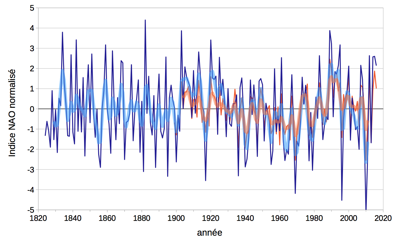
蓝色:标准化压力之间的差异,在直布罗陀和冰岛测量的压力(CRU/UEA数据)。橙色:NCEP 表面压力分析的第一个主要成分(数据来源于J. Hurrell/NCAR)。加粗曲线:11个季节的滑动平均值。[© G. Delaygue]
(annee 年;Indice NAO normalize 标准化NAO指数)

  图2表明,北大西洋南北之间两个连续冬季的压力变率明显(称为年际尺度),但10到20年(10年的尺度)具有持续的趋势。尤其是1900-1910、1920-1930 和 1990-2000 年间,为变化的正位相(称为“NAO+”),指数值呈上升趋势。相比之下,1850-1860和1950-1970(“NAO-”)为负位相。但持续变化过程存在相反方向的极值:例如在正向变化趋势的十年中,1995-1996年冬天的指数是极小值。

3.4. 对天气状况有何影响?

  如上所述,北大西洋地区南北之间的压力转移主要改变了中纬度穿越北大西洋的扰动,以及与这些轨迹相关的西风风速。因此这种转变对天气条件的影响在西欧北部和南部之间是相反的。在夏天,愈加频繁的干扰导致更加潮湿和凉爽的条件。在冬季,则更加潮湿和温和,在北欧通常是下雨而不是干燥寒冷。

环境百科全书-北大西洋涛动-涛动影响a

环境百科全书-北大西洋涛动-涛动影响b
图(3) 1月份NAO+条件的平均影响(NAO指数的月均值。上图:温度异常(ºC)。底图:降水异常(毫米/月)。彩色等值线显示了这些温度和降水异常与年际变率(温度异常标准差为0.8和降水异常标准差为0.5)显著相关的范围。NCEP再分析的1948-2010年数据。
[© G. Delaygue]

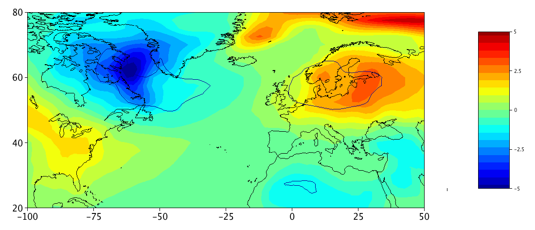
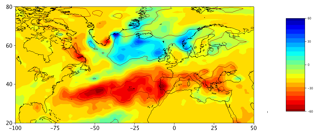
  图3显示出北大西洋涛动对一月典型气象的影响。这些影响不仅限于西欧:由于南北压力转移引起的环流变率,它们还会影响北美东部边缘。拉布拉多地区和斯堪的纳维亚半岛之间的温度存在强烈的遥相关,美国东海岸与地中海和北非(远至近东)之间存在平稳的遥相关。可以注意到,活动中心的温度没有受到影响,而中心是天气波动的驱动因素。降水异常具有“带状”的空间结构,南北差异类似于压力变率,极端值出现在活动中心。

  然而与两个连续冬季的波动(年际变率)相比,温度和降水的影响相对较小,尤其是对降水而言。图 3 中的彩色等值线定义了这些受影响的区域。因此NAO 模态最多只能描述20%到30%的年际温度变率。

  但是北大西洋涛动的这些气象是否影响了欧洲气候?最近发生的一个最好的例子是从20世纪60年代至80年代NAO-到90年代初的NAO+。这种转变是导致西欧变暖的原因,西欧比世界其它区域变暖更迅速,与气候模型的预测值差异明显[6]。这种变暖最明显的影响之一是西阿尔卑斯山的降雪量减少[7]。NAO+持续了大约十年,然后振荡变成了NAO-阶段,有时为极小值(2009-2010年冬季的历史低点)。NAO-阶段伴随着极冷的冬季(2001年12月)和正常的冬季(2004-05、2005-06、2009-10、2010-11)。然而除了这几个寒冷的冬天,法国 2000 年至2010 年期间其他冬天都相当炎热,甚至非常炎热。因此,似乎北大西洋涛动对天气条件的影响较小。各种研究模拟了欧洲的天气状况,同时考虑了移动(包括 NAO 阶段):研究表明自20世纪90年代后期以来,实际天气状况比预期的要温暖,包括21世纪初的寒冷冬季[8]

4. 其他区域的大气组织方式

  在19-20世纪,气象学为揭示区域之间的相关性,对比了所有可用的测量。由于北大西洋涛动,北大西洋盆地很快就被认为是一个具有强烈遥相关的地区。但是其他地区也出现了组织大气的方式。这就是热带太平洋著名的南方涛动 (SO)。通过研究印度季风这一对印度相当重要的现象,吉尔伯特·沃克在20世纪初强调南方涛动。这种振荡与强大的ENSO现象有关(参见 ENSO 文章-准备中)。

  从20世纪80年代开始,大气模型的数据同化技术发展迅速(参见气象资料同化)。 这些模型的分析提供了大气循环及其变异性的全球数据。还可以使用不同的统计工具(例如主成分分析)进一步探索其组织。因此在中高纬度地区确定了影响整个半球的模式,其组织模式被称为“环形”,在极区和周围的中纬度地区(环形结构)之间存在压力变率。它们是北半球环状模(NAM),通常称为北极涛动 (AO),以及南半球环状模(SAM)。

  在北半球环状模中,大西洋地区起着主要作用,大气环流的变异性非常高,同时组织也非常明显。此外,该地区并不总是与北半球的其他地区相同。由于这些原因,北大西洋涛动显然是一种特殊的区域模式。

  一般来说,这些模式描述了大气环流的时间尺度,范围从周(同步)到季节。 北大西洋涛动在几年内也显示出一些持续性,与大气变率速率长时间相关。为了解释这种持续性,气候学家将目光投向了海洋。事实上,海洋表面有一个比大气高得多的热惯性(我们称海洋为“热飞轮”),洋流速度也远低于风。因此这个行星的热飞轮是某些模式(例如 NAO)数十年持续趋势的合理解释。

  对海洋表面温度的研究确定了几种特定于海洋的模式。北半球是大西洋多年代际振荡(AMO),它描述了北大西洋盆地的温度异常。太平洋年代际振荡(PDO),它描述了北太平洋东部和西部地区之间的温度变率。热带地区以“厄尔尼诺/拉尼娜”模式为主,这是 ENSO 模式的一个组成部分,描述了赤道太平洋东部和西部之间的温度异常变率(参见:ENSO 文章 – 准备中)。

  事实上,这种用海洋“飞轮”来解释 NAO十年的持续性的想法已被证明比

  预期的要困难。理论研究[9]表明,大气环流的同步波动(一周左右)是被表层海洋过滤以产生数年的海洋温度和/或环流异常。研究表明影响大气的北大西洋涛动是造成大西洋数十年涛动的原因。与预期相反!因此,20世纪90年代的NAO+阶段是自其中期以来北大西洋变暖的起源,对应于多年代际大西洋的过渡振荡到正相位。这种温暖的大西洋异常现象可能是造成 2010 年欧洲温暖的气候状况的原因。

5. 结论:NAO 的起源和预测潜力

  经过一个世纪对北大西洋涛动的研究,结果如何呢?首先,它是北大西洋盆地大气环流的一个特殊组织形式,有两个相反的阶段(NAO+与NAO-),在冬季尤为明显。大气的数字模型很好地再现了这种组织。但是,由于该组织的因素,有时这两个阶段之间会突然过渡,一个阶段的十年持续时间尚未被明确确定。在周尺度上,热带地区似乎是通过波束在大气层中的传播引起相变的。在季节尺度上,特别是在冬季,考虑到高纬度地区的地表状态和高层大气,似乎可对 NAO相位作出最好的预测。另一方面,即使海洋的“惯性飞轮”效应仍然是一个很好的解释,在十年尺度上的持续趋势仍难以解释。

  最后,北大西洋地区可能是气象学家和气候学家研究最多的地区之一,其测量时间序列最长,也是一个受热带、北极、东部太平洋,甚至平流层等影响强烈的地区。50多年来,即使只是北大西洋涛动,且这个地区的社会影响非常广泛,预测大气环流的季节演变仍然是一个挑战[10]


参考资料及说明

封面图片:Pixabay。

[1] Indicator:Economic losses from climate-related extremes, accessed on 17/02/2017.

[2] 该项目由著名的罗伯特·菲茨罗伊领导,他是达尔文号的探险家和船长。

[3] Stories by missionary Saabye of the contrasting conditions between Greenland and Denmark during the period 1770-78, cited by van Loon & Rogers (1978), Monthly Weather Review, 106, 296-310

[4] Teisserenc de Bort (1883) Study on the winter of 1879-80 and research on the influence of the position of the major centres of atmospheric action in abnormal winters. Annales de la Société Météorologique de France, 31, 70-79; Hildebrandsson & Teisserenc De Bort (1907) Les bases de la météorologie dynamique, Gauthier-Villars, Paris.

[5] Walker & Bliss (1932). World weather V, Mem Royal Meteorol Soc, 4(36), 53-84.

[6] van Oldenborgh et al. (2009). Western Europe is warming much faster than expected. Climate of the Past 5: 1-12, DOI: 10.5194/cp-5-1-2009. Delworth et al. (2016) The North Atlantic Oscillation as a driver of rapid climate change in the Northern Hemisphere. Nature Geoscience 9: 509-512, DOI:10.1038/ngeo2738

[7] Beniston (2012). Is snow in the Alps receding or disappearing? WIRes 3: 349-358, DOI: 10.1002/wcc.179

[8] Yiou et al. (2007). Inconsistency between atmospheric dynamics and temperatures during the exceptional 2006/2007 fall/winter and recent warming in Europe. Geophys Res Lett 34:L21808. DOI: 10.1029/2007GL031981

[9] Frankignoul & Hasselmann (1977). Stochastic Climate Models 2 Application to Sea-Surface Temperature Anomalies and Thermocline Variability. Tellus, 29, 289-305.

[10] Woollings (2010). Dynamical influences on European climate: an uncertain future. Philosophical Transactions of the Royal Society of London 368: 3733-3756, DOI:10.1098/rsta.2010.0040


The Encyclopedia of the Environment by the Association des Encyclopédies de l'Environnement et de l'Énergie (www.a3e.fr), contractually linked to the University of Grenoble Alpes and Grenoble INP, and sponsored by the French Academy of Sciences.

To cite this article: DELAYGUE Gilles (March 14, 2024), 气候变率:以北大西洋涛动为例, Encyclopedia of the Environment, Accessed July 27, 2024 [online ISSN 2555-0950] url : https://www.encyclopedie-environnement.org/zh/climat-zh/climate-variability-example-north-atlantic-oscillation/.

The articles in the Encyclopedia of the Environment are made available under the terms of the Creative Commons BY-NC-SA license, which authorizes reproduction subject to: citing the source, not making commercial use of them, sharing identical initial conditions, reproducing at each reuse or distribution the mention of this Creative Commons BY-NC-SA license.