Drag suffered by moving bodies
PDF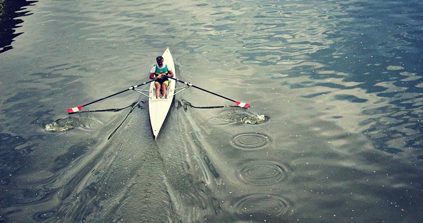
Why does a swimmer have so much difficulty moving through the water? Why do large ships consume so much energy to overcome water resistance? And in such light air, how can birds, cyclists, cars and airplanes overcome this resistance to advancing called drag. It is also this resistance due to the viscosity of the surrounding air that prevents droplets of mist and other small particles from falling (this is called viscous drag). For vehicles or other large objects, the drag is called turbulent: it is related to the loss of energy due to the movement of the displaced fluid. As for surface ships, they also lose energy through another mechanism, this time related to gravity, since waves are generated by the bow lifting the water from which the ship takes its place.
1. Viscous drag: examples of fog and rain
1.1. The viscous friction
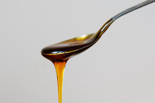
Imagine a flat object, as thin as a razor blade, moving in its plane within a viscous fluid such as honey or oil (Figure 1). Even at low speeds, an effort must be made to advance this plate against resistance due to fluid friction. Locally, each surface unit of this plate is subjected to a tangential force that opposes movement. This friction force is proportional to the viscosity of the fluid (see article Fluids and solids) and the velocity gradient present in the immediate vicinity of the wall.
At the scale of the entire plate, it is the result of these local forces that constitutes the drag resistance force that can be described as viscous as long as other contributions to friction do not mask this effect. This is the case of a spoon falling into the honey, or a smooth, tapered boat hull in slow motion. The flow is then called laminar, which means that each fluid particle follows its own current line, without encroaching on those of its neighbours. This behaviour is different from the turbulent regime discussed below.

The viscous drag of a small sphere is given by Stokes’ formula [1] according to which the drag F is proportional to the diameter d of the sphere and its velocity U with respect to the surrounding fluid, F = 3πµdU The same law applies for honey, water, air, or any other ordinary fluid (called Newtonian) taking into account its dynamic viscosity µ. The same type of formula actually applies to any small object in slow motion, the coefficient 3π being the only element specific to the spherical shape. As expected for friction, drag is always a force aligned with the speed of the object, and in the opposite direction.
1.2. The speed limit of a small object in free fall
In a vacuum, under the effect of gravity, any object, lead or feather, falls with the same uniformly accelerated movement (see the article The laws of dynamics). In a fluid such as water or air, it is also subjected to Archimedes’ thrust, which is none other than the result of hydrostatic pressure forces (see the article Archimedes’ thrust and lift). This force is equal to and opposite to the weight of the displaced fluid, so that the object will fall with reduced acceleration, or rise, depending on whether it is heavier or lighter than the surrounding fluid.
But the object does not accelerate indefinitely because the drag increases with its speed, until it exactly compensates for the driving force resulting from its weight and Archimedes’ thrust. The total force undergone by this object is then zero, as well as its acceleration in accordance with the law of dynamics. The speed that has become constant is called the falling limit speed. It is very quickly reached for a small and light object that we are considering here. Note that it can go upwards for an object lighter than the ambient fluid, such as a bubble or a drop of oil in water.
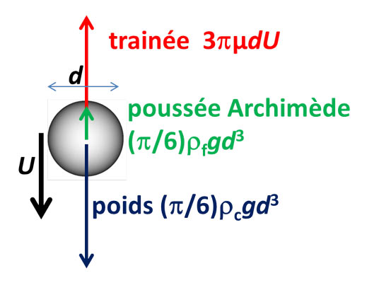
The maximum falling speed can easily be calculated using the Stokes formula given above. Weight is the product of the acceleration of gravity g ≃ 9.81 m.s-2 by the volume of the sphere, (1/6)πd3, and by the density ρc of the body. The Archimedes’ thrust is given by the same formula, using the density of the object ρf of the fluid instead of the body. By cancelling the sum of the three forces (see Figure 3), we can deduce that the maximum falling speed is equal to (1/18)g (ρc-ρf)d2/µ. It is all the lower the higher the viscosity µ is, and it increases as the square of the diameter d. This is why small objects stay in suspension for a long time (see Focus The world of small suspended objects).
1.3. No fog without drag
For example, consider a droplet of mist, which has a diameter of about 20 µm (0.02 mm). Taking into account the density of the water (1000 kg.m-3) and the viscosity of the air (µ = 2 10-5 kg.s-1.m-1), the maximum falling speed of this droplet is about 1 cm.s-1. However, the slightest breath of the surrounding air has a much higher speed. Under these conditions, the droplet remains suspended and moves with the wind. The same applies to pollen grains and all particles smaller than about 20 microns. This explains the long duration of pollution peaks in the calm air of a beautiful high.
The mechanism that causes the fog to disappear, when it occurs, is therefore not its fall to the ground, but its evaporation following sunlight, which may be accompanied by condensation on the ground that remains cold, in the form of dew or frost.
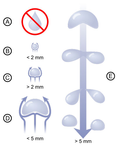
1.4. From fog to rain
In a cloud sufficiently charged with water, the coalescence of the droplets produces larger and larger drops. When their diameter becomes about a millimeter, they fall as rain. If the air flow remained laminar as a drop of diameter d = 2 mm, 100 times larger than a fine droplet of fog, would have a falling speed 10,000 times greater and could reach 100 m.s-1 (360 km/h). In reality, as we will see later, the drag then becomes turbulent, which increases friction and decreases the free fall speed.
2. Turbulent drag
2.1. The Reynolds number
When a large enough body moves in a fluid as low in viscosity as air or water, the flow becomes unstable. This instability is at the origin of the erratic movement of a dead leaf. At higher speeds, a wake of disordered eddies forms downstream of the object, as can be seen at the back of a boat: this is the turbulent wake (see Focus The turbulent wake).
The first scientific characterization of the concept of turbulence was carried out by the Irish physicist and engineer Osborne Reynolds [2]. Its name is attributed to one of the most important ratios in fluid mechanics, called the Reynolds number. This number, noted Re, is equal to the ratio of the time of action of the viscosity (which can be estimated at d2/ν, where ν is the kinematic viscosity [3]) to the transit time of the fluid near the obstacle (near d/U). Its expression is therefore Re = Ud/ν. Turbulence occurs when this Reynolds number exceeds a critical value, always much higher than the unit, which depends on the flow considered.
Although turbulence is a very complex phenomenon, the modelling of which remains problematic, the Reynolds number has the great merit of providing rules of similarity between flows around objects of identical geometric shapes but of different sizes, and with fluids of different viscosities. For example, we can predict that in the same fluid, the wake of an object enlarged by a factor of 10 will become turbulent at a speed 10 times slower. In practice, the wakes of fairly large objects, such as balloons, cars or boats, are always turbulent.
2.2. The drag coefficient
This Reynolds similarity makes it possible to express the turbulent drag according to the expression F = (1/2)CX S ρf U2, where CX is called drag coefficient. This force is proportional to the area S of the maximum cross section swept by the body, also called master torque [4], as well as to the quantities already encountered ρf and U. The CX drag coefficient depends on the shape of the object, but also on the Reynolds number.

This behaviour can be understood by estimating the energy to be expended to set in motion the column of fluid that the body sweeps in its movement [5]. A movement of the entire swept section thus corresponds to Cx ≃ 1, as is the case with the transverse disc. A more streamlined object spreads the fluid less violently, reducing the cross-section of the turbulent wake. The most efficient production cars reach Cx ≃ 0.25. It is in fact the CXS product that controls the drag, which is then easily calculated by multiplying this effective area by the density of the fluid and the square of the velocity.
2.3. A power dissipation proportional to the cube of the speed
The presence of a drag imposes a loss of energy, equal to the work of this force. The corresponding power, or energy lost per unit of time, is obtained by multiplying the drag by the travel speed. Since the force is proportional to U2, the power consumed is proportional to U3. It therefore increases considerably with speed.
This power is converted into the kinetic energy of the fluid (that of all turbulent fluctuations) and eventually dissipates into heat by the action of viscosity. The resulting temperature rise is generally imperceptible because the heat is diluted in a large mass of fluid. However, for a meteorite or spacecraft entering the atmosphere at very high speed, the heating becomes such that it can raise the object’s external temperature to thousands of degrees and lead to its destruction.
2.4. The role of dynamic pressure: drag and lift
While the drag of a slow object is controlled by viscosity, that of a fast object is mainly due to the pressure force induced by the flow, called dynamic pressure. As we have seen, this pressure allows the surrounding fluid to be evacuated laterally from upstream to downstream, so that the moving body can take its place. This difference in pressure causes an overall thrust on the body, which opposes its movement.
At high speed the effect of viscosity becomes negligible, and this overpressure at the stopping point can be estimated at ρfU2/2 using the Bernouilli relationship [6]. Multiplying this overpressure by the transverse area S gives the turbulent drag law stated above. In reality, it is the transverse area of the turbulent wake, in the order of CxS rather than the area S of the object itself, that controls the drag.
In the case of an asymmetric body, such as an aircraft wing or sail, another dynamic pressure force appears, perpendicular to the speed, called lift (see the article Archimedes’ thrust and lift). It is added to the drag, which is aligned with the speed and in the opposite direction. These two forces are proportional to the density of the fluid and the square of the velocity, and their ratio is therefore constant. As we will see later on, this one characterizes the ability of an aircraft to glide: it is called its fineness.
2.5. Some examples of free fall speed limits
In the case of fog and rain, it is easy to estimate the Reynolds number, knowing the kinematic viscosity of the air, ν = 1.5 10-5 m2s-1. For the mist droplet, with d = 20×10-6 m (or 0.02 mm) and U = 10-2 m.s-1, Re ≃ 10-2 is found very clearly in the laminar regime. On the other hand, for the drop with a diameter of d = 2 mm with U = 100 m.s-1, Re = 13 000 is obtained in the turbulent regime. But this falling speed limit is overestimated since it does not take into account turbulent friction. The weight of the drop is (1/6)πgρfd3 = 4 10-5 N, equalizing it with the turbulent drag based on CX = 0.5, one reaches a speed of 6 m.s-1, which gives Re ≃ 800, at the beginning of the turbulent regime.
In the case of a man in free fall, with a mass M = 80 kg, i.e. a weight of 800 N, the drag can be estimated with a section CXS = 1 m2, which gives a speed of 50 m.s-1, i.e. 180 km/h. It takes about 5 s to reach this speed limit, which represents a head (1/2)gt2 ≃ 125 m. The speed limit is thus quickly reached. The jumper then presses his weight on the air and no longer feels any acceleration. Once the parachute is deployed, the speed limit is greatly reduced due to its large transverse area CX S which considerably increases drag by a factor of about 100. The same drag is thus obtained for a speed 10 times lower (because proportional to U2), leading to a limit speed 10 times lower, in the order of 5 m.s-1.
2.6. The importance of fluid density
We have seen that the turbulent drag is proportional to the density of the fluid. At an altitude of 34,000 m, the density of the air is 100 times lower than near the ground; the same drag is then obtained at a speed 10 times higher. The maximum falling speed, for which the drag balances the weight, is therefore 10 times greater, i.e. 500 m.s-1. During his 2012 freefall jump in 2012, from an altitude of 39,000 m, parachutist Felix Baumgartner approached this speed [7], reaching 372 m.s-1 (1,340 km/h), after 45 s of fall, at an altitude of about 30,000 m.
On the other hand, the drag is much larger in water, 800 times denser than air at low altitude, which explains why a solid object falls much more slowly than in air (Archimedes’ thrust also slows the fall, and even cancels it out for an object that floats, but it plays a more limited role than the drag for a dense object such as a stone).
This density effect also explains why a cyclist can reach a speed of 40 km/h, whereas good swimmers rarely exceed 4 km/h. This factor of 10 in speed translates into a factor of 1,000 in power spent (we have seen that it increases as U3). This factor is more or less compensated by the ratio of densities between air and water, so that the power expended is more or less the same in both cases.
3. The gravitational drag on the surface of the water

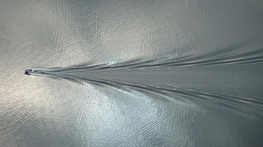
Another effect that slows down the swimming or walking of ships is the wave drag, or gravity drag. The pressure at the tip of the bow exerts a double action. As we have seen, it spreads the upstream water on the sides, from which the ship will take its place. But much of this water is also lifted above the open surface by the bow and falls back on either side of the ship. The potential energy acquired during the uplift (Figure 6) is transformed into kinetic energy during its fall, which extends below the water equilibrium surface. Then, like a pendulum, this water oscillates, rising and falling, while moving away from the ship. This generates the waves seen on the sides of ships as well as those of a swan moving slowly on the calm water of a lake (Figure 7). This gravitational drag transfers part of the energy consumed by the ship to the waves. It is controlled by gravity.

We have seen that viscous and turbulent trails depend on the Reynolds number (Figure 5). The gravitational drag is controlled by another parameter, called Froude number [8], which is expressed as Fr = U /(gl)1/2 where l is the length of the moving object. Experience shows that this drag increases considerably as the number of Froude approaches the unit. The wavelength of the waves produced (distance between two successive ridges) is then close to the length of the boat [9]. The latter spends a considerable amount of energy to ride his own wave, instead of simply lifting the water from the neighbourhood.
4. How to fight the drag?
As small as it is, the trail slows down movement. It can therefore only be maintained if a driving force compensates it. If there is a difference between the driving force and the drag, the body accelerates or slows down, depending on whether the difference is positive or negative. Thus in the case of the free fall discussed above, gravity accelerates the body until the drag accurately compensates for the weight.
Any horizontal movement is regularly slowed down by drag in the absence of power. The horizontal speed of the balls and balloons thus decreases along their trajectory. Their maximum value is imposed by the initial impact (about 260 km/h for a tennis ball or football) and the length of the trajectory then depends on the drag. For example, for a golf ball, the speed record set by world champion Jason Zuback is 320 km/h; the total length of the trajectory was then 400 m. It could have been twice as high in the absence of drag, for a purely ballistic movement subjected to gravity alone.
4.1. The energy cost of speed
A cyclist, even on a horizontal road and without headwinds, must pedal to overcome the resistance to advancing. The transverse area of its CXS wake is between 0.2 and 0.4 m2 depending on its position on the bicycle, more or less upright [10]. Thus for a speed of 15 m/s (54 km/h), the drag will be between 27 and 54 N, and the power to be provided by the cyclist to fight it (obtained by multiplying this force by the speed) is 400 to 800 W. To this must be added the power expended to fight against the mechanical friction of the machine, which is almost independent of speed. Only exceptional champions can maintain power [11] of 400 W beyond a few minutes (in comparison, the average power supplied by a horse is estimated at 735 W, the value of the horsepower). This explains why the cycling hour record is precisely 54 km (Bradley Wiggins in 2015). Limiting your speed to 12 m/s (43 km/h) requires half the power, which is more accessible.
For a well-profiled production car, the CXS product reaches a value of about 0.6 m2. At a speed of 28 m.s-1 (100 km/h), this leads to a drag of 280 N, or 8 kW of power used to overcome the aerodynamic drag alone. This remains modest for an average car, with a typical power of 50 kW. On the other hand, reaching 200 km/h requires fighting a trail 4 times stronger. The energy to be expended for a given path, equal to the product of force and displacement, is therefore 4 times greater. Since the displacement is then twice as fast, the power required (i.e. the energy expended per unit of time), is 8 times greater, i.e. 64 kW instead of 8 kW to compensate for the aerodynamic drag alone. This is only accessible to high-powered cars.
4.2. Different propulsion modes
The rower of the cover image, while pushing the water back with his paddles, releases eddies whose trace on the free surface is clearly visible. Here, it is a drag force that is applied to the oars and pushes the boat forward. The same applies to pedal boats and old wheel boats.
In the case of an aircraft, it is the propellers or engines that provide the propulsion force. Each propeller blade is profiled like an aircraft wing and is therefore subjected to a lift directed perpendicular to its rotational speed. It is designed with additional torsion to effectively direct the propeller thrust forward. In the case of reactors, it is a large number of propellers housed in a fairing that optimizes their operation.
In the case of birds in beaten flight, it is the effort of their muscles that produces a flapping of their wings and provides both the lift and propulsion required, thanks to the release of a vortex at each flapping (Read the article Archimedes’ thrust and lift). Swimmers’ beats, with or without fins, also release eddies in their wake; it is this mechanism that explains their propulsion. It is also a form of lift perpendicular to the movement of the flapping fins or wings.
4.3. The gliding flight

As we have seen, lift and drag are proportional to the square of the speed, and their ratio, called fineness, also represents the inverse of the descent slope in resting air, as shown in Figure 10. It is then the component of the weight Mg projected along the trajectory that pushes the glider, while its transverse component is compensated by the lift, as if the glider was descending on an inclined plane. The most efficient glider bird, the albatross, has a glide ratio of 20, which is similar to that of airliners such as the Airbus A320, with a glide ratio of 17. Modern gliders do better, with a fineness of about 50. In resting air, such a glider can cover a horizontal distance of 100 km for a loss of altitude of only 2,000 m.
The speed of a flying object is thus imposed by the constraint that the lift must balance the weight, with however a possible adjustment range by the angle of incidence with respect to the trajectory. A light and large glider can fly slowly and take advantage of rising winds to rise. On the other hand, to go faster, an aircraft will have to be designed with a smaller wingspan, at the cost of higher energy consumption. Another strategy is to fly higher: at an altitude of 10,000 m, the density of the air is three times lower than on the ground, so that the same drag and lift forces, proportional to the square of the speed, are achieved for a speed multiplied by √3 ≃ 1.73.
5. Towards greater efficiency
5.1. Inspired by animals
Observation of the animal world shows remarkable examples of adaptation to flight or swimming, to minimize drag. Some dolphins are thus able to maintain a speed of 30 km/h, so that we have long sought mysterious mechanisms to suppress turbulence through the flexibility of their skin. But more recent research shows that it is essentially the optimal shape of their bodies, and their exceptional muscle power [12] that gives them these impressive abilities.
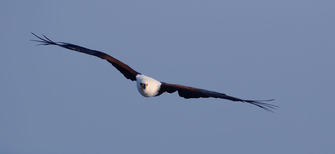
As for birds, they know how to reduce their drag by retracting their legs into their plumage and lying as far as possible in the direction of their trajectory. The majestic gliding flight of the osprey (Figure 9) illustrates well how these birds have developed their know-how and anatomy to minimize their efforts.
5.2. Controlling turbulence

Since turbulence is an essential factor controlling drag, extensive research is being conducted to reduce its effects. This can be achieved by using passive elements such as roughness or scratches, or active elements to prevent the growth of turbulent disturbances. However, there are practical and economic constraints to the development of these systems. In the case of aircraft, a known solution to limit drag is to reattach the air threads to the rear of the wings and fuselage by sucking them through a multitude of small holes; however, this is not implemented due to maintenance problems related to plugging the holes. In liquids, it is possible to reduce turbulent drag remarkably by adding polymers, even in minute concentrations. But this is of course limited to industrial applications in closed environments, for example for pipelines.
In the case of racing boats, the use of foil lift has allowed spectacular progress by freeing itself from the gravity drag. The application to transport ships is much more problematic. The search for speed always represents a significant cost in energy, which is difficult to offset by efficiency gains.
References and notes
Cover image. The drag suffered by the canoe must be compensated by the effort of the rower. The balance of these forces determines the speed of the canoe [Source: pixabay].
[1] George Gabriel Stokes, an Irish physicist who was responsible for the modern formulation of viscosity effects (1819-1903).
[2] Osborne Reynolds, (1842-1912) was an Irish engineer and physicist to whom important contributions to fluid dynamics are due, including the identification of hydrodynamic instabilities using an ink net (Proc. Roy. Soc. London, 35, 84-99, Jan. 1883), in an experiment is still cited today.
[3] The dynamic viscosity of a fluid, often noted at μ, is relevant for evaluating the viscous frictional force. It is counted in kg.m-1.s-1, a unit sometimes called poiseuille, in homage to the 19th century French physician and physicist Jean-Louis Marie Poiseuille. In the study of the effects of viscosity on flow, it is often preferable to use the kinematic viscosity of the fluid ν=µ/ρf, the ratio between its dynamic viscosity and its density (see the article Diffusion and propagation in air at rest). This is counted in m2s-1.
[4] Strictly speaking, the word “torque” refers to the straight section of a hull, the “master torque” being the largest section of all. It is therefore a word from marine vocabulary that we use here to designate the equivalent size about any body or vehicle moving in a fluid.
[5] In a time dt, it scans a cylinder of length Udt and section S, thus a mass ρfSUdt. To communicate the velocity U to this mass requires the contribution of kinetic energy ½ ρfSU3dt, which must be the work of the friction force FUdt. This leads to the formula of the drag force with Cx=1.
[6] Daniel Bernoulli (1700-1782), a Swiss doctor, physicist, mathematician and philosopher, professor at the University of Basel, was particularly interested in the study of fluid flow. Bernoulli’s theorem, published in 1738 in the book Hydrodynamica, plays a fundamental role in fluid mechanics. It requires that p+ρfu2/2= p0 along a power line, where p is the local pressure and p0 its value at the upstream stop point where the velocity cancels out (we are placed in the reference linked to the body).
[7] It then exceeded the speed of sound, which provides additional braking force: the energy of the fall is no longer used only to spread the air around the body, but to compress it and emit a shock wave, a high amplitude sound wave, the famous sound wall. This wave drag is also well known for boats, but this time by the emission of waves, governed by gravity.
[8] This number is named after William Froude (1810 -1879), a British engineer and naval architect who was at the origin of the first scientific studies of gravity drag.
[9] The Froude number physically represents the ratio between the boat’s U speed and the speed of wave propagation in deep water, which depends on their wavelength l per c=(gl)1/2 . The wake waves follow the boat as it moves, and for this to happen, they must propagate at the same speed as the boat. The relationship c≃U then leads to a first estimate of the wavelength of the wake, and this reaches the length of the boat when the Froude number is equal to 1.
[10] See http://sportech.online.fr/sptc_idx.php?pge=spfr_xfd.html
[11] This mechanical power supplied corresponds to a total power consumed by the body of about 1.9 kW, the efficiency being about 21%, see http://www.agoravox.fr/culture-loisirs/sports/article/puissance-et-performance-en-159520. This power consumed is related to the quantity of oxygen captured by the breath.
[12] F.E. Fisch and G.V. Lauder, 2006, Ann. Rev. Fluid Mech. https://www.yumpu.com/en/document/view/46389631/passive-and-active-flow-control-by-swimming-fishes-and-mammals.
The Encyclopedia of the Environment by the Association des Encyclopédies de l'Environnement et de l'Énergie (www.a3e.fr), contractually linked to the University of Grenoble Alpes and Grenoble INP, and sponsored by the French Academy of Sciences.
To cite this article: MOREAU René, SOMMERIA Joël (January 5, 2025), Drag suffered by moving bodies, Encyclopedia of the Environment, Accessed July 12, 2026 [online ISSN 2555-0950] url : https://www.encyclopedie-environnement.org/en/physics/drag-suffered-moving-bodies-2/.
The articles in the Encyclopedia of the Environment are made available under the terms of the Creative Commons BY-NC-SA license, which authorizes reproduction subject to: citing the source, not making commercial use of them, sharing identical initial conditions, reproducing at each reuse or distribution the mention of this Creative Commons BY-NC-SA license.