Climate models

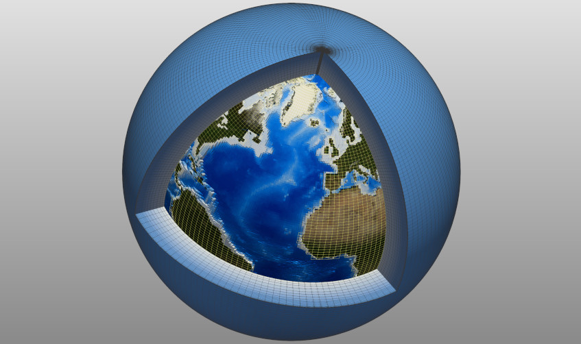
What are climate models? On what basis are they built? How are they evaluated? Are they reliable? How is the climate of the future explored? This article attempts to answer these questions by highlighting the limitations of these models and the scientific questions they raise. Climate models are a valuable tool for understanding the climate and anticipating future changes. Above all, they constitute a digital laboratory that allows scientists to explore the complex processes that make up the climate system. Projections made with these models follow common protocols that allow the simulations produced by different models to be compared rigorously. In this way, we can quantify the modelling uncertainty in climate projections.

1. A climate model consists of several components

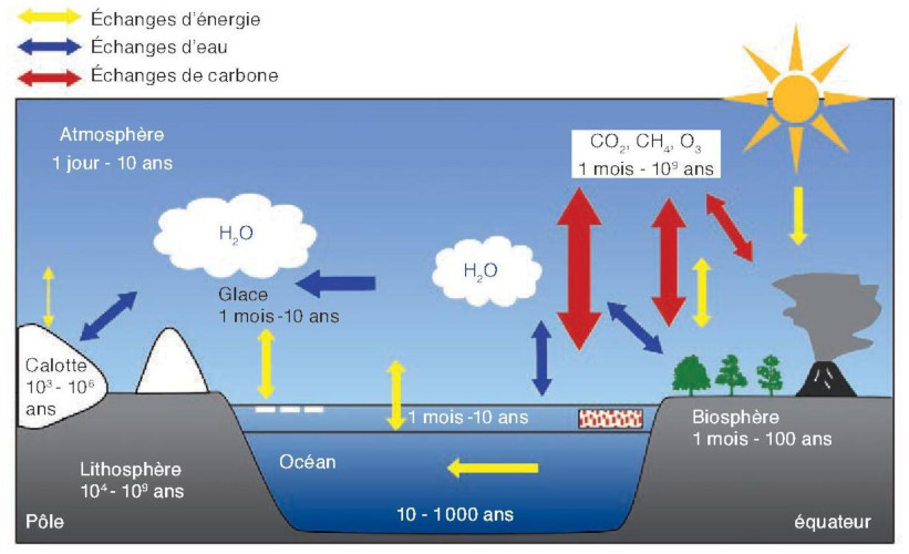
A climate model is a numerical representation of the climate system (read: The Climate Machine). The climate models described here are the models used to make climate projections for the next century and are constructed to represent the processes at play on a scale of a few centuries. These models represent all the components of the climate system that change at these times-scales: atmosphere, ocean, cryosphere and biosphere (Figure 1) [1]. In the models, the different components are usually developed separately and can be used alone or coupled together.

1.1. Ocean and atmosphere

The ocean and atmosphere components are based on the equations of fluid mechanics and thermodynamics as well as on the principles of mass [2] and energy conservation. To transcribe these equations into numerical form, the globe is cut into small cubes, the meshes (Figure 2) [3] and the temporal progression is done in successive time steps. Numerical methods for representing the fluid mechanics differential equations can vary from model to model depending on whether the emphasis is on the accuracy of the calculations or their efficiency. These equations are used to determine the average of the climatic parameters (temperature, humidity, etc.) on each mesh at each time step. Ocean models are built according to the same principles, taking into account the different properties of water compared to air. In particular, water is more viscous than air.

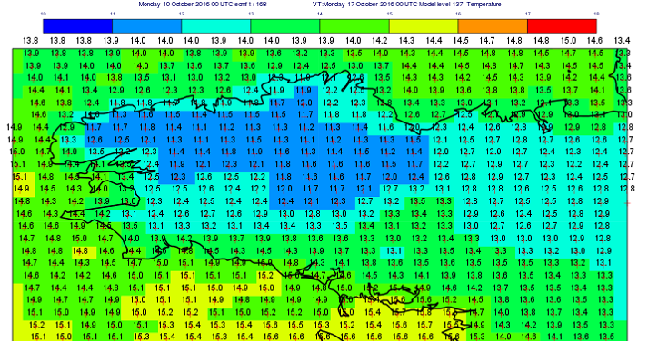
In climate simulations, the size of a mesh is of the order of a hundred kilometres, and the time step is a few tens of minutes. Intra-grid processes, such as cloud formation or precipitation formation, cannot therefore be represented directly by fluid mechanics equations. However, these processes must be taken into account: in order to represent them, parameterizations are used which aim at reproducing in an empirical way the effects of these processes on the scales solved [4]  by the dynamics equations.

Atmospheric models include parameterizations for radiation penetration into the air, for turbulence, convection, cloud and precipitation formation, cloud interactions with radiation, etc. Ocean models also contain parameterizations to represent radiation penetration into the water, mixing related to smaller scale eddies, tide-induced mixing and turbulence. Parameterizations are also used to represent transfers of water, energy and momentum between the ocean and the atmosphere. Parameterizations are equations written empirically from observations. These equations are universal in a given model, in the sense that they are the same at any point on the globe.

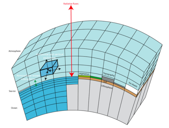
The atmospheric models used for climate simulations are thus constructed in the same way as weather forecasting models. The difference stems from the length of time these models are integrated and the way in which their results are interpreted (see Part 3). In general, global weather prediction models divide the Earth’s atmosphere into grids of a few kilometres on the sides and a few hundred metres vertically. To reduce the cost of calculation, climate models use larger meshes (seeFigure 2) [3], especially on the horizontal dimension, which makes it possible to integrate them over several decades or even centuries. Even if the meshes are larger, climate models represent many successions of meteorological phenomena such as rain, drought, the passage of depressions, etc.

1.2. Continental surfaces

Continental surface models aim to represent the exchange of water and energy between the soil, the biosphere and the atmosphere. They are based on energy and water conservation principles. For example, an area of forest will capture more solar energy because it is darker (its albedo is lower) than an area covered with pasture. On the other hand, if the surface soil is dry, a tree will be able, thanks to its deeper roots, to use water in the deep soil and produce a flow of water to the atmosphere by evapotranspiration, while grasses will not be able to do so. These models also represent seasonal snow on the ground as well as frost in the soil. As in atmospheric models, many processes take place at scales smaller than the mesh size and need to be parameterized.

1.3. Sea-ice and Ice scheets

Sea-ice models represent the exchanges of water, salt and energy between the sea-ice and the ocean, but also between the ice pack and the atmosphere. In these models, the ice pack moves as a function of near-surface winds and ocean currents. These movements lead to sea ice piling up in some areas and divergence [5] in others.

The ice sheet models included in climate models are generally very simplified and are primarily intended to represent the effect of ice cover on the land, but their extent does not vary. More complex ice sheets models already exist, particularly for the Arctic and Antarctic ice sheets, but they require the atmospheric parameters to be represented with finer grids than in current global climate models. Their coupling with climate models is one of the current challenges of climate modelling and becomes crucial for very long-term climate simulations (several centuries).

1.4. Coupling of components

In climate models, the different components are coupled: they evolve together, interacting with each other. In general, continental surface models and atmospheric models interact at each time step of the atmospheric model (a few minutes). Exchanges between ocean models and atmospheric models take place at least once a day or even hourly depending on the model.

2. An adaptable level of complexity

2.1. Complexity

To make realistic climate projections, climate models must describe the four components of the climate system: atmosphere, ocean, biosphere and cryosphere. The complexity of a model is thus defined as the number of climate processes taken into account. The first climate models developed in the 1970s represented only the atmospheric component. Models evolved rapidly and managed to include all four components by the late 1990s. Since then, the models have constantly improved by refining existing parameterizations and adding the representation of new processes. For example, most current models represent the life cycle of particles in suspension in the atmosphere, called aerosols See Air pollution). The models thus represent their transport by winds, their interaction with cloud formation processes and their leaching by rain.

The most complex models represent the entire carbon cycle, and make it possible to estimate carbon exchanges between the different components. These exchanges themselves depend on climate, the properties of seawater and the ability of vegetation and the marine biosphere to convert carbon into organic matter.

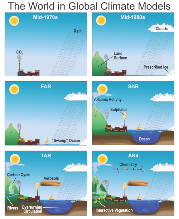
There are also very simplified, one-dimensional models based on the terrestrial radiation balance, which simulate only the global mean temperature and not regional disparities. However, in order to represent the effect of an increase in carbon dioxide concentration in these simple models, they will need information from the full models described above. Between these highly simplified energy balance models and the full models, there is a range of models of increasing complexity (Figure 3), developed for specific applications.

2.2. Adaptation to use

The most complex models are also more costly in terms of computing time. However, depending on the study being carried out, it is not necessary to take all these processes into account. In particular, the inclusion of the full representation of the carbon cycle relies on parameterizations that are still uncertain and whose feedbacks may be important. In order to study the impact of a given increase in atmospheric carbon dioxide concentration on climate processes such as El Niño phenomena, for example, it is preferable to use a model without representation of the carbon cycle, whose results will be easier to interpret. The results will then help to understand the projections of the carbon cycle model. It is therefore sometimes necessary to decouple the questions.

Thus, the most complex model is not necessarily the most suitable for all uses. With the level of complexity, more degrees of freedom are also introduced into the system. This complicates its calibration and validation, sometimes at the expense of model robustness. The interpretation of the results is also more delicate. Moreover, the more complex the model, the more powerful the computers required and the longer the computation time. However, in order to carry out studies on the climate machine, it is often necessary to carry out several tests before reaching reliable conclusions. It is therefore important that the calculation cost is reasonable in order to be able to carry out many tests.

2.3. Costs calculation

The cost of running a climate model increases with the complexity and with its resolution, i.e. the size of the meshes. The calculation cost also depends on the numerical methods used to represent the model equations. Thus, the cost of a current climate model varies from a few dozen calculation days to a thousand to simulate a year if only one processor is used. This is why these models are implemented on supercomputers, among the most powerful machines in the world. By using a large number of processors simultaneously, the simulation of a year can be done in a few hours. For example, it takes several weeks to make a simulation of a 100-year climate projection. The volumes of data produced are also very large, of the order of a few hundred Gigabytes (GB) per simulation year, or a few dozen Terabytes (TB) for a 100-year simulation.

A climate model is a numerical laboratory for testing hypotheses, as can be imagined in biology with test tubes. In biology, the same treatment is often repeated on several individuals to verify its effectiveness on a panel of tests. Similarly in climate, it is often appropriate to carry out the simulations in the form of ensembles. As the climate system is chaotic, it is sometimes difficult to separate the climate changes that are due to imposed forcing, for example an increase in greenhouse gases, from the internal variability of the climate system (read: Climate variability: the example of the North Atlantic Oscillation). Simulation sets subject to the same forcings but with slightly different starting states are then performed to determine the robust impacts of the applied forcings. The less numerically expensive the model, the larger the size of the ensembles that can be performed and the more confidently the results can be interpreted.

2.4. Regionalization

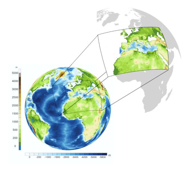
The calculation cost also determines the mesh size of the climate models. Currently, these meshes are on average 100 km x 100 km, although some models manage to reach a few tens of km². This spatial resolution makes it possible to represent many phenomena such as the succession of perturbations in the mid-latitudes, or tropical monsoons. On the other hand, these global models do not allow the representation of more local phenomena, such as cyclones and regional circulations directly linked to the topography. Thus, in a climate model with a resolution of 100 km, the topography is too smooth for the Rhône valley to be represented distinctly, and this prevents Mistral episodes from being represented in the model.

To carry out studies on finer resolution phenomena, a regional climate model can be used, as is done in weather forecasting. The finer-grid regional model will need to be “guided” at the boundaries of its domain by a global climate model (Figure 4). Regional models are built on the same principles as global models (similar algorithms, same process). They can themselves be more or less complex. Some represent only the atmospheric component, but there are also coupled regional ocean-atmosphere models. Such models thus make it possible to study smaller-scale phenomena, but the results depend on both the regional model used and the global model used at the boundary of the domain. It is therefore important to take account of this double uncertainty, for example by carrying out a set of regional simulations forced by several global models.

3. How is a climate model validated?

3.1. Component validation

A climate model is validated in successive stages. Each component of the model is developed independently of the others by applying observations as input variables. Within this constrained framework, it is verified that the model produces realistic results. Thus, a land surface model will be used alone by providing meteorological observations as input variables and it will be verified that the temperature, soil moisture and vegetation evolve in accordance with the observations.

Each component is thus adjusted and assessed separately from the others. Each component is also used for studies specific to its environment. In this step, a few model parameters can be considered to be unconstrained by available observations and the range of acceptable values for these parameters will be assessed. These parameters can eventually be adjusted within this range once the complete model is assembled. During the steps constrained by observations, the simulation results can be directly compared with observations in terms of time evolution.

3.2. Input data

When simulating with a climate model, there are two types of input data: initial state and forcings. While in weather forecasting, the initial state is a key input, in climate modelling, forcings are the most important input. The main forcings are: greenhouse gas concentrations (except water vapour, simulated by the atmospheric component), aerosol load, but also the distribution of vegetation, volcanic eruptions and solar energy received at the top of the atmosphere. Because the climate system is chaotic, information from the initial state is quickly lost. The initial conditions are therefore of little importance for climate simulations over several decades.

However, the memory of the climate system is longer than that of a weather prediction model, because the oceans evolve less rapidly than the atmosphere and this inertia lengthens the memory of the system. It is this property that is used to make forecasts on a seasonal scale. Seasonal forecast models are climate models in which the atmosphere and ocean components are initialized based on observations. They take advantage of the fact that the ocean has significant inertia to forecast trends over the coming months. These systems are much less reliable than weather forecasting models but provide relevant information on the evolution of phenomena such as El Niño in particular and on tropical variability in general. Hindcasting over a large number of past years allows a seasonal forecasting system to be tested and is a form of model validation. However, this type of validation is limited to periods of a few months, which is still short compared to the climatic time-scales.

The use of climate models to predict somewhat longer time horizons of a few years is a current research topic [6]. Some studies consider predictability [7] to be possible up to one or two years. Beyond a few years, initial conditions are of little importance and applied forcings become dominant.

3.3. Validation of the complete system

The chaotic nature of the climate system has important consequences on how to validate a complete climate model. A simulation lasting several decades, even when forced by observed forcings, will not follow the chronology of observations due to this chaotic nature (and model imperfections). Even if the model were perfect, it would not be able to follow the sequence of weather events as they occur. It will therefore not be possible to compare the evolution of the temperature over a country in relation to the observations. On the other hand, the model will be able to represent the climatological characteristics of the climate (Figure 5) [8]: the seasonal cycles of temperature and precipitation averaged over 30 years can be compared with the (average) climatology of the observations. Similarly, long-term trends can be compared with those of the observations. For example, the models show the reduction in spring snow cover at mid-latitudes during the 20^th century [9].

Validation is not only about long-term climate characteristics. It will also assess the model’s ability to adequately represent the daily variability of precipitation, i.e. its ability to represent the number of dry days and very wet days in a given season at a given location around the globe. The model’s ability to represent extreme events, such as storms, can also be assessed (see Extreme weather events and climate change).

This validation step determines the limits of these models. For example, they are often able to represent the distribution of different types of clouds around the globe, but for the most part, they currently fail to adequately represent the thin stratocumulus-type clouds on the eastern edges of the tropical oceans, such as off Chile, California or Angola [10]. When simulations of future climate are analysed, these shortcomings will have to be taken into account as a limitation of model reliability in these regions. The validation step also indicates the processes by which the modellers need to improve the models to make them more reliable.

Climate models thus produce information on all time scales (Figure 1), from the diurnal cycle to trends at the century scale. Models are therefore evaluated on their ability to represent many processes at all these temporal and spatial scales. It is from the physical consistency of the whole that our confidence in these models emerges. Downstream of the modelling activity, the work of climate researchers thus consists of processing large masses of data using appropriate statistical methods.

4. Climate projections, what assumptions are made?

To make climate projections, modellers must prescribe, as input data for climate models, the forcings over the coming century.

For solar radiation and volcanoes, it is difficult to predict their level of future activity. So simple assumptions are made. For solar radiation, the last observed 11-year cycle is reproduced periodically over the next century [11]. For volcanoes, only their average effect is considered for the future without variations (but more specific studies are carried out to address this issue).

For other forcings, greenhouse gases, aerosols and land use change, their evolution is highly dependent on the evolution of human activities. These forcings are referred to as anthropogenic forcings. Economists provide different scenarios (Figure 6) of how these forcings will change based on demographic and economic assumptions. Economists use specific models for this purpose, known as “integrated impact models [12]“.

Several types of evolution are envisaged, depending on whether or not the population becomes aware of the risk and adapts its practices, depending on demographic changes and whether or not regions are turning in on themselves. Economists thus produce several types of scenarios for changes in greenhouse gas concentrations. The scenario that will actually be followed remains uncertain, and it is important to consider several forcing scenarios when looking at climate projections.

Climate models are then integrated over the 21^st century by varying forcings under these economic scenarios. The initial conditions are derived from simulations of the 20^th century and intrinsically incorporate the effect of forcings over past periods.

Depending on the level of complexity of the model, the type of forcing is adapted. For example, for models that do not represent the carbon cycle, CO₂ concentrations will be prescribed to the model. Conversely, if the model represents the carbon cycle, the model will apply anthropogenic carbon emission forcings, with natural emissions being dynamically represented in the model. Similarly, for models that do not include a life-cycle representation of aerosols, the climate model will be prescribed concentrations of these particles, which are themselves derived from specific models forced by the chosen economic scenario.

5. IPCC and model intercomparison exercises

5.1. The IPCC

The Intergovernmental Panel on Climate Change (IPCC) regularly produces reports that aim to summarize the state of scientific knowledge on climate, its evolution, impacts and ways to adapt to projected changes. In order to coordinate the work of the various teams implementing climate models around the world, a model intercomparison exercise (Coupled model intercomparison project -CMIP) is carried out upstream of the IPCC reports. The aim of these exercises is to propose common experimental protocols to the modelling centres that will make it possible to study climate change and characterise the uncertainty associated with modelling in a rigorous manner.

The CMIP project also provides modelling centres with storage space and tools to share the data produced by the models. These databases are public [13] and can be used by researchers around the world to conduct climate change studies. For the next IPCC report due in 2021, 29 teams have published data from 54 different models (as of 04/03/2020). Many centres are implementing several models by playing with the complexity of the model and/or its spatial resolution.

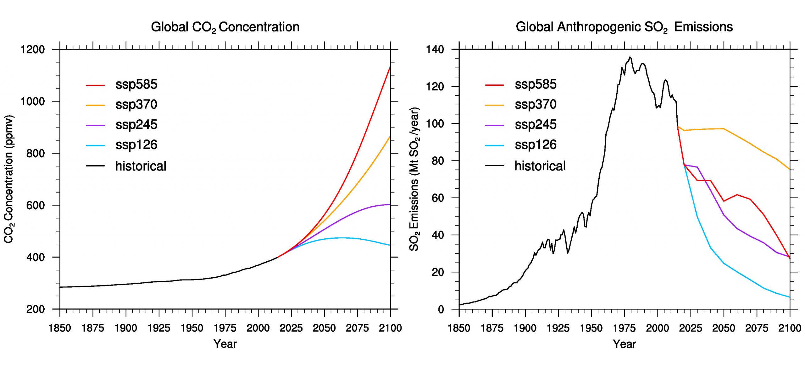
5.2. Future forcing scenarios

For this sixth exercise (CMIP6), 4 scenarios of changes in greenhouse gases and main aerosols were used to force the models (Figure 7):

• A scenario with very limited concentrations, called ssp126, which requires a reduction in emissions from the middle of the century and negative emissions from 2080 onwards;
• A scenario with an increase in emissions at the current rate, ssp585, which forecasts CO₂ concentrations of 1135 ppm in 2100;
• Between these two extremes, the ssp245 scenario, which represents an intermediate future where societies partially adapt, and the ssp370 scenario, an intermediate with a higher concentration but with the particularity of forecasting a lower reduction in aerosol emissions.

For the previous exercise (CMIP5, Figure 7) [14], by comparing the projections of all models under a given scenario, modelling uncertainty (as distinct from scenario uncertainty) can be assessed. This is about 1.6°C for the worst-case scenario, which projects a global temperature change of 4°C as a multi-model average compared to the end of the 20^th century. It is well understood that the total uncertainty results both from uncertainty about the future of demographics and the economy (scenario) and from uncertainty about the evolution of the climate forced by anthropogenic emissions.

In order to better compare the models with each other, climate modellers have defined a more theoretical metric, called climate sensitivity, which corresponds to the increase in surface temperature after a doubling of CO₂ concentration compared to the pre-industrial era. This is the change in temperature at equilibrium, which implies that the model must be integrated long enough for the global surface temperature to stabilize. This theoretical quantity allows us to compare the magnitude of the feedbacks that appear in the climate system following an increase in CO₂  concentration. Indeed, the first impact of CO₂ is to warm the air locally, but this warming has multiple consequences, called feedbacks. For example, if the air warms up, the Clausius-Clapeyron relationship indicates that it will be able to hold more water vapour. This can have impacts on cloud formation, cloud position, etc. It is the relative importance of these different feedbacks that is uncertain and the study of several models allows a better understanding of them.

For the last exercise (CMIP6), the uncertainty between models has rather increased [15]; in particular a dozen models simulate an equilibrium sensitivity that exceeds the range of 1.5°C-4.5°C established by the previous IPCC report and which had already been considered by the Charney report in 1979 [16]. These initial results are based on the analysis of a reduced number of models and will need to be verified when data from more models become available. The reasons for this increase in sensitivity for some models are the subject of intense research. Several studies also attempt to use recent observations to constrain sensitivity estimates. It is indeed crucial to determine whether such strong values are plausible.

Climate models are thus laboratory tools to better understand processes within the climate system and to advance knowledge. However, it should not be forgotten that these models are imperfect. It is necessary to compare them with observations in order to understand their limitations and continuously improve them.

6. Messages to remember

• A climate model is a numerical representation of the climate system.
• Climate models are of varying degrees of complexity. The complexity is chosen according to the scientific objective of the study.
• Climate models allow future climate projections to be made, but these are based on scenarios of economic and demographic changes.
• The uncertainty of the projections results both from the uncertainty of the climate modelling but also from the uncertainty of the economic and demographic evolution.
• A climate model is a valuable laboratory tool for advancing our understanding of the climate system.

---

Notes and References

Cover image. Diagram representing the atmosphere as seen by a numerical model: a cutting into small cubes. [Source : © CEA 2020 / Realisation: P. Brockmann (LSCE)]

[1] Joussaume S. (2011) Le climat : un thème de recherche pluridisciplinaire ; dans “Le climat à découvert“, Jeandel C. & Mosseri R. (Eds.), CNRS Editions.

[2] Mass of dry air for the atmosphere, salt for the ocean and water for all components.

[3] Goosse H., P.Y. Barriat, W. Lefebvre, M.F. Loutre & V. Zunz, (06/06/2020). Introduction to climate dynamics and climate modeling. Online textbook available at http://www.climate.be/textbook.

[4] Solved scale: scale of time and space represented by the fluid dynamics equations which is inherently larger than the mesh of the models.

[5] Divergence: indicates that dynamic tends to export ice to other regions. For example, along a coast if sea ice is transported offshore by local winds, the ice will tend to disappear or become thinner at the coast.

[6] Boer, G. J., Smith, D. M., Cassou, C., Doblas-Reyes, F., Danabasoglu, G., Kirtman, B., Kushnir, Y., Kimoto, M., Meehl, G. A., Msadek, R., Mueller, W. A., Taylor, K. E., Zwiers, F., Rixen, M., Ruprich-Robert, Y., and Eade, R. (2016). The Decadal Climate Prediction Project (DCPP) contribution to CMIP6, Geosci. Model Dev, 9, 3751-3777, doi: 10.5194/gmd-9-3751-2016.

[7] Predictability: Predictability measures the ability to predict with respect to the target time frames under the assumption that the initial state is well known.

[8] Hai-Tien Lee and NOAA CDR Program (2018): NOAA Climate Data Record (CDR) of Monthly Outgoing Longwave Radiation (OLR), Version 2.7. NOAA National Centers for Environmental Information. https://doi.org/10.7289/V5W37TKD [2020-05-29]

[9] Brown, R. D. and Robinson, D. A. (2011) Northern Hemisphere spring snow cover variability and change over 1922-2010 including an assessment of uncertainty, The Cryosphere, 5, 219-229, doi: 10.5194/tc-5-219-2011.

[10] Zuidema, P., et al (2016) Challenges and Prospects for Reducing Coupled Climate Model SST Biases in the eastern tropical Atlantic and Pacific Oceans: The US CLIVAR Eastern Tropical Oceans Synthesis Working Group, B. Am. Meterol. Soc, doi: 10.1175/BAMS-D-15-00274.1.

[11] Cyclicity simulated from reconstructions over 9400 years for CMIP6 (Matthes et al., 2017), available at https://solarisheppa.geomar.de/cmip6

[12] O’Neill, B. C., Tebaldi, C., van Vuuren, D. P., Eyring, V., Friedlingstein, P., Hurtt, G., Knutti, R., Kriegler, E., Lamarque, J.-F., Lowe, J., Meehl, G. A., Moss, R., Riahi, K., and Sanderson, B. M. (2016) The Scenario Model Intercomparison Project (ScenarioMIP) for CMIP6, Geosci. Model Dev, 9, 3461-3482, doi: 10.5194/gmd-9-3461-2016.

[13] Earth System Grid Federation

[14] Knutti, R., & J. Sedláček (2012) Robustness and uncertainties in the new CMIP5 climate model projections. Nat. Climate Change 3, 369-373, doi:10.1038/nclimate1716

[15] Zelinka, M. D., Myers, T. A., McCoy, D. T., Po-Chedley, S., Caldwell, P. M., Ceppi, P., et al. 2020. Causes of higher climate sensitivity in CMIP6 models. Geophysical Research Letters, 47, e2019GL085782. doi: 10.1029/2019GL085782.

[16] National Research Council. 1979. Carbon Dioxide and Climate: A Scientific Assessment. Washington, DC: The National Academies Press. doi: 10.17226/12181.