气候模式

  什么是气候模型？它们是基于什么而建立的？如何对它们进行评估？他们是否可靠？如何探索未来的气候？本文试图通过强调这些模型的局限性以及它们所提出的科学问题来回答这些问题。气候模型是理解气候并预测未来气候变化的非常有价值的工具。最重要的是，它们构成了一个数字实验室，使科学家能够探索构成气候系统的复杂过程。用这些模型做出的预测遵循共同的协议，允许对不同模型产生的模拟进行严格的比较。通过这种方式，我们可以量化气候预测模型的不确定性。

1. 气候模型的组成部分

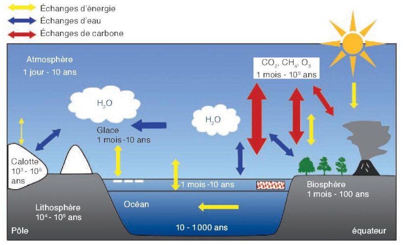
  气候模型是气候系统的数字表现形式（参见：“气候机器”）。这里所描述的气候模型是用于对下个世纪进行气候预测的模型，旨在表达几个世纪以来正在发生的气候变化的过程。这些模型代表了这些时间尺度上发生变化的所有气候系统：大气、海洋、冰冻圈和生物圈（图1）[1]。在模型中，不同的部分通常是单独开发的，可以单独或结合在一起使用。

1.1. 海洋与大气

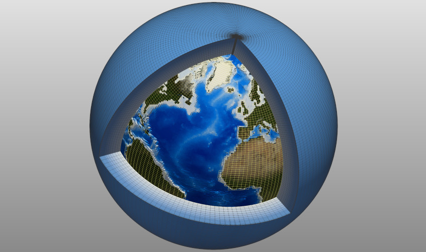
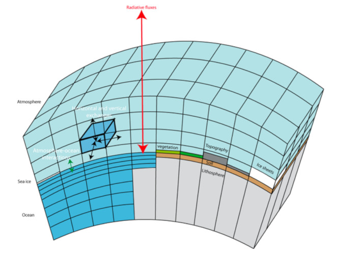
  海洋和大气分量是基于流体力学和热力学方程式以及质量[2]和能量守恒的原理建立的。为了将这些方程式转化为数值形式，地球被切割成小立方体，网格(图2)和时间级数是在连续的时间序列中完成的。表示流体力学微分方程的数值方法可能因模型而异，这取决于重点是计算的准确性还是计算的效率。这些方程用于确定在每个时间步长中每个网格上的气候参数（温度、湿度等）的平均值。海洋模型是根据相同的原理构建的，并考虑到了水与空气不同的特性，特别是水比空气更粘稠。

  在气候模拟中，每个网格的大小约为一百公里，时间步长为几十分钟。因此，网格内的过程（例如云或降水的形成）不能用流体力学方程直接表示。但是，这些过程又必须被考虑。为了描述它们，使用了参数化的方法，以一种经验/半经验方程的形式描述这些过程在格点尺度上的影响[4]。

  大气模型包括辐射的参数化过程，湍流、对流、云和降水形成过程，云与辐射的相互作用等。海洋模型还包括辐射穿透到水中，与小尺度涡流有关的混合，潮汐引起的混合和湍流的参数化过程。参数化还用于表示海洋与大气之间水、能量和动量的传递。参数化是根据观察经验得出的在给定的模型中是通用的方程，从某种意义上说，它们在地球上的任何地方的应用都是一样的。

  因此，用于气候模拟的大气模型与天气预报模型的构造方式相同。二者差异在于模型的积分时间长短以及结果的解释方式（请参阅第3部分）。总的来说，全球天气预报模型将地球的大气层划分为宽度几公里，垂直几百米的网格。为了减少计算成本，气候模型使用较大的网格（请参见图2）[3]，尤其是在水平尺度上，这使得它们模拟数十年甚至几个世纪的大气特征。即使网格较大，气候模型也能代表许多连续的天气现象，例如降雨、干旱、气旋等。

1.2. 陆地表面

  陆面模型旨在代表土壤，生物圈和大气层之间水和能量的交换。它们基于能量和水分守恒原则。例如，森林区域相较于草场覆盖的区域会吸收更多的太阳能，因为森林区域的颜色更暗（反照率较低）。另一方面，如果表层土壤干燥，在深根系的作用下，树木将能够利用深层土壤中的水，并通过蒸散作用将水输送到大气，而草无法做到这一点。这些模型还能描述陆地上的季节性降雪以及土壤中的霜冻。与大气模型一样，许多过程发生在比网格尺寸小的尺度上，需要进行参数化。

1.3. 海冰和冰盖

  海冰模型代表了海冰与海水之间以及浮冰与大气之间的水、盐和能量的交换。在这些模型中，浮冰的移动是近地表风和洋流的函数。这些移动导致一些地区海冰堆积，而另一些地区则发生了海冰破碎[5]。

  气候模型中包含的冰盖模型通常都非常简化，主要是为了表示冰盖对陆地的影响，但其范围没有变化。但是针对北极和南极冰盖，冰盖模型更复杂，与目前的全球气候模型相比，它们需要用更精细的网格来表示大气参数。它们与气候模型的耦合是当前气候建模的挑战之一，对于长期的气候模拟（几个世纪）而言变得至关重要。

1.4. 模型组分耦合器

  在气候模型中不同的组成部分是相互耦合的：它们同时演变，彼此相互作用。通常，陆面模型和大气模型在其每个时间步长（几分钟）上都会相互作用。海洋模型和大气模型之间的交换每天至少发生一次甚至每小时一次，这主要具体取决于模型的设计。

2. 模式适用性的复杂程度

2.1. 模式的复杂程度

  为了尽可能做出真实的气候预测，气候模型必须描述气候系统的四个组成部分：大气、海洋、生物圈和冰冻圈。因此，将模型的复杂性定义为模型涉及的气候过程的数量。20世纪70年代开发的第一个气候模型仅代表大气分量。随着模型的迅速发展，并在20世纪90年代后期已经包含了所有四个组成部分。从那时起，通过细化现有的参数并加入新的气候过程，模型得到了不断的改进。例如，目前大多数模型都反映了悬浮在大气中的微粒，即气溶胶（aerosols，参见：“空气污染”）的生命周期。因此，这些模型可以描述它们在风中的传输，它们与云形成过程的相互作用以及降雨的湿沉降作用。

  用来模拟完整碳循环的模型最为复杂，这类模型使估算不同组分之间的碳交换量成为可能。这些交换本身取决于气候、海水的性质以及植被和海洋生物将碳转化为有机物的能力。

  还有非常简化的基于地面辐射平衡的一维模型，该模型仅模拟全球平均温度但不能显示区域差异。但是，为了在这些简单模型中描述二氧化碳浓度增加带来的影响，他们也需要来自上述完整模型的信息。在这些高度简化的能量平衡模型和完整模型之间，存在针对特定应用而开发的一系列复杂性不断提高的模型（图3）。

2.2. 模式的适用性

  就计算时间而言，最复杂的模型计算成本也更高。但是，正在进行的研究表明模型中考虑所有的气候过程是没有必要的。特别是，碳循环的完整表述依赖于仍然不确定的参数化，而这些参数化的反馈可能很重要。例如，为了研究给定的大气二氧化碳浓度增加对厄尔尼诺Niño现象等气候过程的影响，最好是使用不涉及碳循环的模型，其结果将更容易解释。这些结果将有助于理解碳循环模型的预测。因此，有时有必要将这些问题分离开。

  因此，最复杂的模型并不一定适合所有用途。随着复杂程度的提高，模型系统也引入了更多的自由度。这使它的校准和验证变得复杂，有时会以牺牲模型的稳定性为代价。结果的解释也更加微妙。而且，模型越复杂，所需的计算机越强大，计算时间就越长。然而，为了对气候机理进行研究，往往需要进行几次测试，才能得出可靠的结论。因此，合理的计算成本是非常重要的，以便能够执行多次测试。

2.3. 模式的计算成本

  气候模型的运行成本随着其复杂性及其分辨率（即网格的大小）的增加而增加。计算成本还取决于用于表示模型方程的数值方法。因此，如果仅使用一个处理器，当前气候模型模拟一年的气候变化的计算成本从几十个到上千个计算日不等。这就是为什么要在世界上功能最强大的超级计算机上实现这些模型并行运算的原因。通过同时使用大量处理器，一年的模拟可以在几个小时内完成。例如，要模拟100年的气候预测需要花费几周的时间。模拟过程中数据的生成量也非常大，每个模拟年大约产生数据百千兆字节（GB），而对于100年的模拟则大约需要几十TB。

  气候模型是用于检验假设的数字实验室，就像生物学实验中使用试管一样。在生物学中，通常对多个个体重复相同的处理，以通过一组实验验证其有效性。同样，在气候方面通常以集合形式进行模拟。由于气候系统是混乱的，有时很难将外力（例如温室气体增加）所引起的气候变化与气候系统的内部变率区分开来（阅读：“气候变率：以北大西洋涛动为例”）。模拟集合受到相同的外力，但启动状态略有不同，然后执行模拟，以确定所施加外力的强大的影响。模型的数值成本越低，可以执行的集合规模就越大，对结果的解释也越自信。

2.4. 区域化

  计算成本也决定了气候模型的网格大小。尽管某些模型的精度可以达到几十km²，但目前这些网格的平均大小仍为100 km x 100 km。这种空间分辨率已经可以表示许多现象，例如中纬度或热带季风的持续干扰。另一方面，这些全球模型不能描述更多局部现象，例如气旋和与地形直接相关的区域环流。因此，在分辨率为100 km的气候模型中地形太过平坦，无法清晰地表现小尺度的山谷，使得山谷风在模型中无法被模拟。

  为了对更高分辨率的气候现象进行研究，可以像天气预报一样使用区域气候模型。精细网格的区域模型需要在其边界上由全球气候模型进行“引导”（图4）。区域模型建立原则与全球模型相同（相似的算法和相同的过程），它们本身的复杂性可以自行把握。一些模型仅包含大气分量，但也有一些模型耦合了区域海洋-大气模型。因此，此类模型使得研究较小规模的现象成为可能，但是结果既取决于使用的区域模型也取决于在域边界使用的全球模型。因此考虑到这种双重不确定性是非常重要的，例如可以通过执行由多个全球模型强迫的一组区域模拟来降低这种不确定性。

3. 如何验证气候模式？

3.1. 模块验证

  模型的每个模块都是通过将观测数据作为输入变量而独立开发出来的。在这个约束框架内，可以验证该模型产生了真实的结果。因此，将气象观测作为输入变量单独使用陆面模型进行模拟，并验证是否与温度、土壤湿度和植被的观测结果一致。

  因此，每个模块都与其他模块分开进行调整和评估。每个模块还可用于特定环境的研究。在这一步中，可以认为一些模型参数不受现有观测值的约束，并评估这些参数的可接受值范围。一旦完整的模型组装完成，这些参数最终可以在这个范围内进行调整。在受观测值约束的步骤中，模拟结果可以直接与观测值在时间演化上进行比较。

3.2. 数据输入

  使用气候模型进行模拟时有两种类型的输入数据：初始状态和外力。在天气预报中初始状态是关键的输入数据；在气候建模中，外强迫是最重要的输入。主要的外力有：温室气体浓度（水汽除外，由大气成分模拟）、气溶胶浓度，以及植被分布、火山爆发和大气顶接收的太阳能。由于气候系统是混乱的，来自初始状态的信息会很快丢失，所以初始条件对几十年来的气候模拟影响不大。

  但是，气候系统的记忆时间比天气预报模型的记忆时间长，因为海洋的演化速度不及大气快，而这种惯性延长了系统的记忆。我们正是利用这个属性用来进行季节尺度的预测。季节预报模型是基于观测结果对大气和海洋模块进行初始化后的气候模型。他们利用海洋具有很大的惯性这一事实来预测未来几个月的趋势。这些系统的可靠性远不及天气预报模型，但可以提供一些现象演变的相关信息，例如厄尔尼诺现象，以及有关热带变化的信息。对过去多年的追算（Hindcasting）可以对季节性预报系统进行测试，是模型验证的一种方式。但是，这种类型的验证仅限于几个月的时间，与气候预测的时间尺度相比仍然很短。

  使用气候模型预测更长的时间跨度是当前的研究主题[6]。一些研究认为，可预测性可达一到两年。若干年后，初始条件就不那么重要了，而施加的外力就会起主导作用。

3.3. 验证整个系统

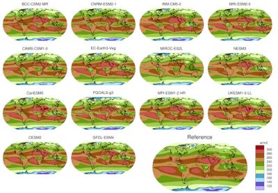
  气候系统的混沌性质对如何验证一个完整的气候模型具有重要影响。即使是在观察到的外力作用下，因为这种混沌的性质（以及模型不完善），持续数十年的模拟也不会遵循观测的时间顺序。即使模型是完善的，也将无法跟踪天气事件的发生顺序。因此，不可能将一个国家的温度变化与观测结果相比较。另一方面，该模型将能够表示气候的平均特征（图5）[8]：30年平均温度和降水的季节循环可以与观测的（平均）气候学数据进行比较。同样，可以将长期趋势与观察结果进行比较。例如，模型表明20世纪中纬度地区春季积雪覆盖的减少[9]。

  验证不仅涉及长期气候特征。它还评估模型所能表示降水日变化的能力，即全球给定位置给定季节中干燥天数和潮湿天数的能力。还可以评估模型表示极端事件（例如风暴）的能力（参见：“极端气候和气候变化”）。

  这个验证步骤决定了气候模型的局限性。例如，它们通常能够表示全球不同类型的云的分布，但在大多数情况下，目前还不能充分表示热带海洋东部边缘的薄层积云的形成，如智利、加利福尼亚或安哥拉[10]。当分析这些对未来气候的模拟结果时，必须考虑这些缺点，作为这些地区模型可靠性的限制。验证步骤还指明了建模者需要通过哪些过程来改进模型，以使它们更可靠。

  因此，气候模型会产生从日周期到世纪尺度的所有时间尺度的信息（图1）。因此，对模型的评价取决于它们在所有这些时间和空间尺度上表示多过程的能力。正是从整体的物理一致性中，我们对这些模型产生了信心。所以在建模工作的下游，气候研究人员的工作还包括使用适当的统计方法处理大量数据。

4. 气候预测有哪些假设？

  为了做出气候预测，建模者必须指定未来一个世纪的外力作为气候模型的输入数据。

  对于太阳辐射和火山，很难预测它们未来的活动水平。因此做出简单的假设，对于太阳辐射，最近观测到的11年周期将在下个世纪周期性地重现[11]。对于火山，未来仅考虑其平均作用，而不会考虑变化（但针对此问题进行了更具体的研究）。

  对于其他外力，如温室气体，气溶胶和土地利用的变化，其演变高度取决于人类活动的变化。这些外力称为人为外力。经济学家基于人口和经济对这些外力的影响假设提供了不同的情景（图6）。经济学家为此使用了特定的模型，即“综合影响模型”[12]。

  根据是否意识到人口风险并调整策略，同时根据人口变化和各区域是否正在自我转变，大家设想了几种演变类型。因此，经济学家提出了几种温室气体浓度变化的情景。然而实际将要遵循的情景仍然不确定，在查看气候预测结果时，必须考虑几种外力情景。

  然后通过这些经济情景下不同的外力将21世纪的气候模型进行整合。初始条件是从20世纪的模拟中得到的，并且在本质上包含了过去的外力的影响。

  根据模型的复杂程度，可以调整外力类型。例如，对于不包含碳循环的模型，将在模型中指定CO₂浓度。反之，如果模型包含碳循环部分，则该模型将应用人为碳排放作为外力，而自然排放则在模型中动态表示。同样，对于不包含气溶胶生命周期的模型，气候模型将规定这些颗粒的浓度，这些颗粒浓度本身是来源于选择的经济情景使用特定的模型计算得到的。

5. IPCC和模式比对工作

5.1. IPCC

  政府间气候变化专门委员会（IPCC）定期发布报告，旨在总结有关气候的科学知识状况、气候演变、影响以及适应预测变化的方法。为了协调在世界各地实施气候模型的各个团队的工作，在IPCC报告的上游进行了模型比较工作（耦合模型比对项目Coupled model intercomparison project -CMIP）。其目的是向建模中心提出通用的实验方案，这将使研究气候变化和表征与建模相关的不确定性成为可能。

  CMIP项目还为建模中心提供了存储空间和工具，以共享模型产生的数据。这些数据库是公开的[13]，可供世界各地的研究人员用来进行气候变化研究。在2021年应提交的IPCC报告中，有29个团队发布了54种不同模型的数据（截至2020年3月4日）。许多中心通过利用模型的复杂性和/或其空间分辨率来实现几个模型的耦合。

5.2. 未来的外力强迫情景

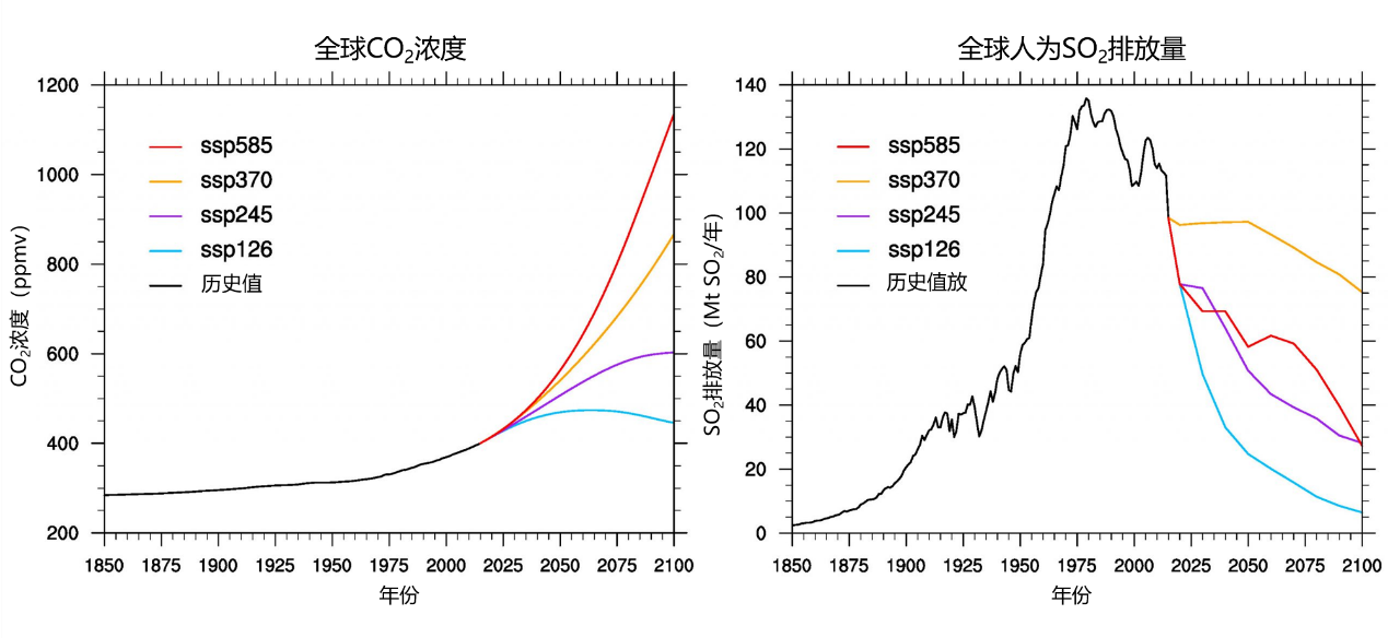
  对于第六次模式对比项目（CMIP6），采用了温室气体和主要气溶胶变化的4种情景来强制模式运行（图7）：

• ssp126是一种浓度非常低的方案，要求从本世纪中叶开始减少排放并从2080年开始负排放；
• ssp585是一种以当前速率增加的排放方案，该方案预测2100年的CO₂浓度为1135 ppm；
• 在这两个极端情景之间，ssp245情景代表了社会部分适应的中间未来情景，而ssp370情景是一种浓度较高但具有预测气溶胶排放减少较少的特殊性的中间情景。

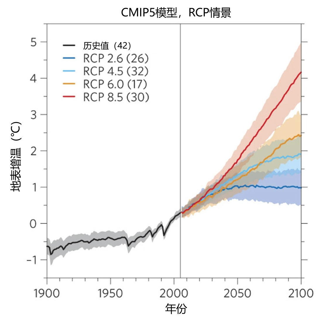
  先前的耦合模型比较项目（CMIP5，图7）[14]通过比较给定情景下所有模型的预测，以评估模型不确定性（不同于情景的不确定性）。根据多模型预测结果，相较于20世纪末全球温度将发生约1.6℃到4℃的变化。众所周知，这种不确定性源于对未来人口和经济（情景）的不确定性以及对人为排放所导致的气候演变的不确定性。

  为了更好地将模型进行比较，气候建模人员定义了一个更理论化的指标，称为气候敏感度，它对应于CO₂浓度比工业化以前增加一倍后地表温度上升的程度。这是平衡时的温度变化，这意味着该模型必须经过足够长的时间才能使全球表面温度稳定下来。这一理论上的数值使我们能够比较CO₂ 浓度增加后气候系统中出现的反馈的强度。确实，CO₂的第一个影响是局部使空气变暖，但是这种变暖会有多种后果，称为反馈。例如，如果空气变暖，则克劳修斯-克拉佩龙（Clausius – Clapeyron）关系表明它将能够容纳更多的水蒸气。这可能会影响云的形成，云的位置等。这些不同反馈的相对重要性是不确定的，研究几个模型可以更好地理解它们。

  最近的一次对比项目（CMIP6），模型之间的不确定性已经相当大[15]；特别是十几个模型模拟的平衡敏感度超过了先前IPCC所报告的建立在1.5°C-4.5°C范围，1979年Charney的报告中已经考虑过这一范围[16]。这些初始结果基于对较少的模型数量的分析，当更多模型的数据可用时则需要进一步进行验证。对于某些模型来说，这种敏感度增加的原因是一个深入研究的课题。一些研究还试图利用最近的观测来约束敏感性的估计。确定这些巨大的价值是否可信确实至关重要。

  因此，气候模型是用来更好地了解气候系统内的过程并推进知识的实验工具。但是，我们不应忘记这些模型并不是完善的。有必要将它们与观察结果进行比较，以了解其局限性并不断加以改进。

6. 要点

• 气候模式是气候系统的数字表示。
• 气候模式具有不同程度的复杂性，复杂度是根据研究的科学目的进行选择的。
• 气候模式允许对未来的气候做出预测，但是这些预测都是基于经济和人口的变化情况。
• 预测的不确定性不仅来自气候模式的不确定性，还来自经济和人口发展的不确定性。
• 气候模式是促进我们对气候系统了解的宝贵的实验工具。

 

---

参考资料及说明

封面图片：用数值模型表示大气图示：地球被切成小立方体 [来源：© CEA 2020 / Realisation: P. Brockmann (LSCE)]

[1] Joussaume S. (2011) Le climat : un thème de recherche pluridisciplinaire ; dans “Le climat à découvert“, Jeandel C. & Mosseri R. (Eds.), CNRS Editions.

[2] Mass of dry air for the atmosphere, salt for the ocean and water for all components.

[3] Goosse H., P.Y. Barriat, W. Lefebvre, M.F. Loutre & V. Zunz, (06/06/2020). Introduction to climate dynamics and climate modeling. Online textbook available at http://www.climate.be/textbook.

[4] Solved scale: scale of time and space represented by the fluid dynamics equations which is inherently larger than the mesh of the models.

[5] Divergence: indicates that dynamic tends to export ice to other regions. For example, along a coast if sea ice is transported offshore by local winds, the ice will tend to disappear or become thinner at the coast.

[6] Boer, G. J., Smith, D. M., Cassou, C., Doblas-Reyes, F., Danabasoglu, G., Kirtman, B., Kushnir, Y., Kimoto, M., Meehl, G. A., Msadek, R., Mueller, W. A., Taylor, K. E., Zwiers, F., Rixen, M., Ruprich-Robert, Y., and Eade, R. (2016). The Decadal Climate Prediction Project (DCPP) contribution to CMIP6, Geosci. Model Dev, 9, 3751-3777, doi: 10.5194/gmd-9-3751-2016.

[7] Predictability: Predictability measures the ability to predict with respect to the target time frames under the assumption that the initial state is well known.

[8] Hai-Tien Lee and NOAA CDR Program (2018): NOAA Climate Data Record (CDR) of Monthly Outgoing Longwave Radiation (OLR), Version 2.7. NOAA National Centers for Environmental Information. https://doi.org/10.7289/V5W37TKD [2020-05-29]

[9] Brown, R. D. and Robinson, D. A. (2011) Northern Hemisphere spring snow cover variability and change over 1922-2010 including an assessment of uncertainty, The Cryosphere, 5, 219-229, doi: 10.5194/tc-5-219-2011.

[10] Zuidema, P., et al (2016) Challenges and Prospects for Reducing Coupled Climate Model SST Biases in the eastern tropical Atlantic and Pacific Oceans: The US CLIVAR Eastern Tropical Oceans Synthesis Working Group, B. Am. Meterol. Soc, doi: 10.1175/BAMS-D-15-00274.1.

[11] Cyclicity simulated from reconstructions over 9400 years for CMIP6 (Matthes et al., 2017), available at https://solarisheppa.geomar.de/cmip6

[12] O’Neill, B. C., Tebaldi, C., van Vuuren, D. P., Eyring, V., Friedlingstein, P., Hurtt, G., Knutti, R., Kriegler, E., Lamarque, J.-F., Lowe, J., Meehl, G. A., Moss, R., Riahi, K., and Sanderson, B. M. (2016) The Scenario Model Intercomparison Project (ScenarioMIP) for CMIP6, Geosci. Model Dev, 9, 3461-3482, doi: 10.5194/gmd-9-3461-2016.

[13] Earth System Grid Federation

[14] Knutti, R., & J. Sedláček (2012) Robustness and uncertainties in the new CMIP5 climate model projections. Nat. Climate Change 3, 369-373, doi:10.1038/nclimate1716

[15] Zelinka, M. D., Myers, T. A., McCoy, D. T., Po-Chedley, S., Caldwell, P. M., Ceppi, P., et al. 2020. Causes of higher climate sensitivity in CMIP6 models. Geophysical Research Letters, 47, e2019GL085782. doi: 10.1029/2019GL085782.

[16] National Research Council. 1979. Carbon Dioxide and Climate: A Scientific Assessment. Washington, DC: The National Academies Press. doi: 10.17226/12181.