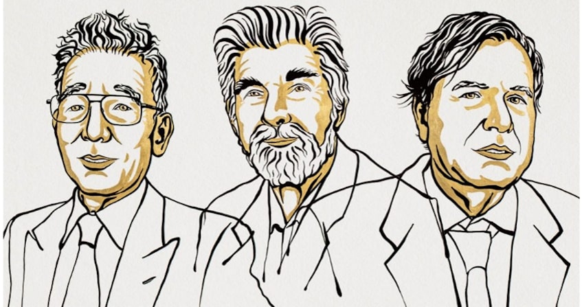
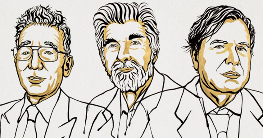
Three laureates share the 2021 Nobel Prize in Physics: Syukuro Manabe and Klaus Hasselmann for “laying the foundations of our knowledge of the Earth’s climate and its influence by human activities ” and Giorgio Parisi for “his revolutionary contributions to the theory of disordered and random phenomena ” as the Swedish Academy of Sciences writes in its justification for awarding the prize. The work of Syukuro Manabe and Klaus Hasselmann is the subject of this article. The work of Giorgio Parisi is presented in the article “On the contributions to statistical physics of Giorgio Parisi, Nobel Prize in Physics 2021” in the physics section of this same encyclopaedia.

What are the contributions for which one half of the 2021 Nobel Prize in Physics was awarded to Syukuro Manabe and Klaus Hasselmann? How was their work on “physical modelling of the Earth’s climate, quantification of variability and reliable prediction of global warming”, as the Swedish Academy of Sciences wrote in its justification of the award, seminal for physical climatology? What do they have in common, what makes them different? What progress has been made since their pioneering work over 40 years ago for Hasselmann and over 50 years ago for Manabe? This article attempts to answer these questions.

1. Introduction: Climate, a complex physical system of primary importance to humanity

The climate is a prime example of a complex physical system. It is governed by fundamental physical, chemical and biological processes that are mostly well understood. But the interaction between many processes and various components of the system (Figure 1), across a wide range of spatial and temporal scales, generates a complex behaviour of the Earth’s climate. This complexity makes it difficult to describe mathematically and to predict, or even understand, its behaviour.

Syukuro Manabe is one of the pioneers of physical climate modelling using computers: it is their computational capacity that makes it possible to represent the interactions between the processes involved and thus to bring out, in the numerical simulation, the characteristic behaviour of the climate system. More than 50 years ago, Manabe and his colleagues laid the foundations for predicting the climate response to greenhouse gas emissions. As we shall see later, this pioneering work has already described the key spatial and temporal features of climate change underway today.

The work of Klaus Hasselmann has provided a better understanding of how a predictable climate system response emerges from chaotic behaviour on short time scales. His essential contribution, in his seminal work of 40 years ago, was to pave the way for the branch of climatology that deals with the detection of climate change and the identification of its causes, and thus its attribution to human or natural causes. His methods of identifying “fingerprints” now allow the IPCC to judge that the dominant role of human nature in the climate change observed over the past 150 years or so is a proven scientific fact.

The contributions of Manabe and Hasselmann are described in turn in a little more detail in the next two sections of this article.

2. Physical Climate Modelling

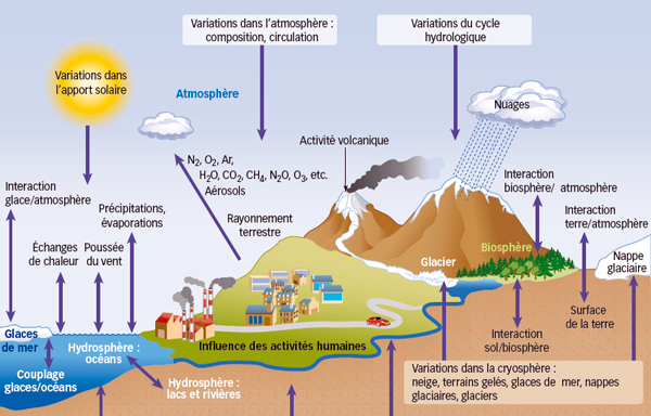
As described in more detail in the article on climate models, physical climate modelling is essentially based on two pillars.

The first pillar consists of the representation of the atmospheric circulation, later extended to the oceanic circulation, typically on the scale of a hundred kilometres. It consists of the solution of the equations of fluid mechanics with a time step of a few minutes. The major weather systems known as “synoptic” and their evolution in time, from hour to hour, are thus explicitly simulated. With the advent of the first computers – and in fact even before that by Richardson [1] – pioneering work [2], [3] was done as early as the 1950s to simulate atmospheric flow. Often the long-term goal was numerical weather prediction rather than modelling of climate change, which at that time was a known but often perceived as less pressing issue (See: Thinking about climate change (16th-21st centuries)).

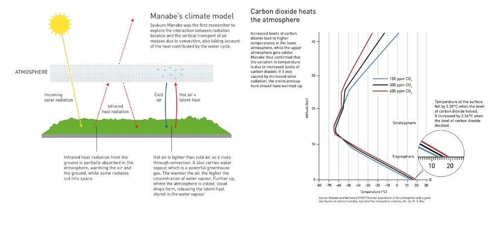
The second pillar is the representation of many other physical, and even chemical and biogeochemical, processes in more recent models. Commonly referred to as ‘the physics’ in the jargon of climate modellers, this includes a representation of processes related to different types of radiation in the atmosphere. Syukuro Manabe’s work is mainly in the area of this second “physics” pillar. His contribution, particularly to the question of the effect of an increase in the concentration of greenhouse gases in the 1960s, was central to the further development of the nascent scientific discipline.

Already at the end of the 19th century, Arrhenius [4] had made calculations based on the radiative properties of CO₂ to answer the question of how much the global average temperature would rise if the concentration of this gas in the atmosphere were to double – a quantity that is now called the climate sensitivity. He estimated this sensitivity at about 5 to 6°C. (Read: From the discovery of the greenhouse effect to the IPCC)

But it was finally Syukuro Manabe who, in a series of three articles [5], [6], [7] succeeded in quantifying this climate sensitivity using a three-dimensional model of atmospheric circulation.

The first work highlighted by the Nobel Prize Committee for Physics (2021), namely the paper by Manabe and Strickler (1964), consisted of developing a one-dimensional model of the atmosphere (a vertical column, Figure 2), in which the vertical temperature profile was calculated as a function of the radiative properties of gases constituting the atmosphere and the moist convective adjustment [8].

The second paper (Manabe and Wetherald, 1967) describes a key improvement to this model (replacing a constant specific humidity profile with a constant relative humidity profile), which allows for the representation of the water vapour feedback – the fact that warmer air can hold more water vapour, thus increasing the greenhouse effect. Thus armed, Manabe and Wetherald were able to use this model to recalculate climate sensitivity. Their result, an increase of 2.3°C for a doubling of atmospheric CO₂, can be considered a key result in the history of climate modelling, if not in the history of climate science.

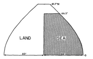
Advances in computer technology allowed Manabe and Wetherald (1975) to use a three-dimensional version of this model. This much more complete version incorporated the full (but simplified) equations of heat, mass, momentum and radiation in the atmosphere; the Earth in this very simple model (Figure 3) was actually represented by a large third of an idealized hemisphere, half continent, half ocean between the equator and 66.5°N, and fully continental beyond, with cyclic looping at the eastern and western edges of the domain; the “ocean” was nothing more than an ever-wet continental surface. Despite these simplifications, this model, run on a computer far less powerful than today’s smartphone, clarified and extended the 1967 results. It made it possible to specify the value of the climate sensitivity obtained in 1967: 2.93°C. Even today, the IPCC [9] places the value of this sensitivity at about 3°C (between 2.5 and 4°C). The 1975 work extended the 1967 results in the sense that it was able to show several important characteristics of the climate change observed today, notably an amplification of climate change at high northern latitudes and an intensification of the hydrological cycle.

Since those pioneering days, the number of climate scientists has increased dramatically, computer computing power has exploded, observations, especially via satellites, have become incomparably more accurate and complete, and climate change, essentially a prediction in the early 1970s, has become an undeniable reality. All of this shows how robust and visionary the work of Manabe (and other pioneers, many of whom are now deceased) was.

3. How to detect climate change within the weather “noise” and how to prove that it is attributable to human activities.

In the 1970s, human-induced climate change could be considered a prediction. As shown in Figure 4, in 1970 the increase in global mean temperature over the beginning of the century was still modest and did not really break through the ‘noise’ of natural (interannual and decadal) climate variability. Nevertheless, in the 1970s, Klaus Hasselmann was able to lay the foundation for what would become the science of climate change detection and attribution.

One of the fundamental characteristics of the climate system is its variability on all time and space scales, starting with meteorological variability. For this reason, any attempt to detect climate change is essentially a question of whether the observed signal – a change in ‘average’ temperature (read: The average temperature of the earth) over a few decades, for example – is outside this ‘noise’ of natural variability. The first work on this issue cited by the Nobel Prize Committee for Physics (2021) is the paper published by Hasselmann in 1976 [10].

In this work entitled “Stochastic climate models”, he uses the analogy of Brownian motion to analyse the variability spectrum of a system coupled between two components, one of which – the atmosphere – is characterised by strong variability on short time scales (this is the domain of meteorology), while the other – the ocean – is more inert. His simple but elegant model shows that the “slow” component, i.e. the ocean, integrates the “white” noise [11] of the atmosphere – i.e. chaotic meteorological variations on all time scales – and then exhibits a spectrum of variability dominated by the slow variations. Since the ocean, with its large surface area and high thermal inertia, is the ‘driving’ component of the climate system on long time scales, this work has allowed us to understand natural climate variability as ‘red’ noise.

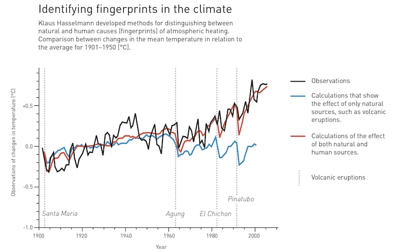
Consider Figure 4 [12]. By comparing observed climate change (black curve) with simulations of a climate model with (red curve) and without (blue curve) human drivers over the period 1900-2020, it is now easy to identify the role of human activities as the main cause of climate change. While the model simulates a realistic climate evolution when it takes into account human factors, the climate it simulates at the beginning of the 21st century in the absence of these human factors is very different from observations. Today, the red and blue curves are unambiguously distinguishable from each other and the impact of human activities emerges very clearly from the noise of the interannual variability. The main contribution of Klaus Hasselmann was to lay the foundations for methods of detecting the ‘fingerprint’ of human-induced climate change in a work published in 1979 [13].

This “fingerprint” [14] is the spatio-temporal structure, but not the magnitude, of the response of a climate model to human forcing (i.e., to increases in greenhouse gas concentration, aerosol emissions, or land use changes). Once these spatial and temporal structures of the responses are known through modelling, we can then ask ourselves how much of the observed climate variations are due to these responses to human forcings. Several statistical methods can be used for this work. Essentially, it is a matter of reconstructing the observed change, in its spatial and temporal characteristics, on the basis of the spatio-temporal structures of the simulated responses to the various human-induced forcings, and not on the basis of the anticipated amplitudes of these responses. For greenhouse gases, it is therefore essentially the climate sensitivity as simulated by the model. The advantages of this approach are many, but perhaps the most important is the high efficiency of the method, allowing reliable attribution of human-induced climate change. As Santer and co-authors [15] aptly wrote “instead of searching for a needle in a tiny corner of a large haystack (and then proceeding to search in the next tiny corner), Hasselmann advocated a more efficient strategy – simultaneous searching of the entire haystack …”

4. Take-home messages

• Klaus Hasselmann paved the way for the detection of climate variations and the identification of their causes by highlighting the dominant role of human activities in the observed warming since the mid-19th century.
• Syukuro Manabe was the author of the first physical model to show the sensitivity of the climate to the CO₂ content of the atmosphere. As early as 1967, a first version of this model predicted an increase in average temperature of 2.3°C for a doubling of the CO₂ concentration. In 1975, a three-dimensional version of this model completed this prediction by predicting the amplification of this warming at northern latitudes, later confirmed by observations.
• While the IPCC was honoured in 2007 with the Nobel Peace Prize, the Nobel Prize for Physics awarded in 2021 is recognition of the considerable progress made in understanding the evolution of the Earth’s climate and current global warming.

---

Notes and References

Cover image. From left to right: Syukuro Manabe, Klaus Hasselmann and Giorgio Parisi. [Source: © Illustration by Niklas Elmehed]

[1] Richardson, L. F. 1922. Weather Prediction by Numerical Process, Cambridge University Press, 250 pp, Cambridge, UK

[2] Charney JG, Fjörtoft R, von Neumann J. 1950. Numerical Integration of the Barotropic Vorticity Equation. Tellus 2 (4), 237-254

[3] Phillips, N. A. 1956. The general circulation of the atmosphere: A numerical experiment, Q. J. Roy. Meteor. Soc. 82, 123-164

[4] Arrhenius A. 1896. On the Influence of Carbonic Acid in the Air upon the Temperature of the Ground, Phil. Mag. 41, 237-275

[5] Manabe, S, Strickler, RF. 1964. Thermal equilibrium of the atmosphere with a convective adjustment J. Atmos. Sci. 21, 361-85

[6] Manabe, S, Wetherald, RT. 1967. Thermal equilibrium of the atmosphere with a given distribution of relative humidity. J. Atmos. Sci. 24, 241-259

[7] Manabe, S, Wetherald, RT. 1975. The Effects of Doubling the CO₂ Concentration on the climate of a General Circulation Model. J. Atmos. Sci. 32, 3-15

[8] Atmospheric convection is the process of vertical movement of air masses induced by density differences, which largely determines temperature and humidity profiles in the troposphere.

[9] IPCC, 2021: Summary for Policymakers. In: Climate Change 2021: The Physical Science Basis. Contribution of Working Group I to the Sixth Assessment Report of the Intergovernmental Panel on Climate Change [Masson-Delmotte, V., P. Zhai, A. Pirani, S. L. Connors, C. Péan, S. Berger, N. Caud, Y. Chen, L. Goldfarb, M. I. Gomis, M. Huang, K. Leitzell, E. Lonnoy, J.B.R. Matthews, T. K. Maycock, T. Waterfield, O. Yelekçi, R. Yu and B. Zhou (eds.)). Cambridge University Press. In Press.

[10] Hasselmann K. 1976. Stochastic climate models part I. Theory. Tellus 28(6), 473-485

[11] In analogy to white light, which is composed of light at all frequencies of equal intensity, “white” noise is a random time series whose frequency spectrum is essentially constant. Similarly, “red” noise is a random time series whose frequency spectrum is dominated by low-frequency variations, in analogy to red light.

[12] https://nobelprize.org/uploads/2021/10/fig4_fy_en_21_fingerprints.pdf, after Hegerl and Zwiers, 2011, Use of models in detection & attribution of climate change.

[13] Hasselmann K. 1979. On the Signal-to-Noise Problem in Atmospheric Response Studies. In: Meteorology of Tropical Oceans. Ed. by D.B. Shaw. London: Roy Meteorol Soc. pp. 251 – 259

[14] By analogy with the fingerprint of each person is unique, it is considered that each factor that influences climate leaves its own fingerprint in terms of climate response (Wikipedia)

[15] Santer, BD et al. 2019. Celebrating the anniversary of three key events in climate change science. Nature Clim. Change 9, 180182